Probability Basics

A hands-on primer with clear theory + simulations and visualizations.

What you’ll learn

Random variables, PMF/PDF/CDF, expectation, variance.
Canonical distributions: Bernoulli, Binomial, Geometric, Poisson, Uniform, Normal, Exponential.
Law of Large Numbers (LLN) and Central Limit Theorem (CLT) via simulation.
Joint & conditional probability, independence, covariance, correlation.
Bayes’ rule with an applied diagnostic-testing example.

How to use this notebook: Read each Theory block first, then run the code cell(s) that follow to build intuition via simulation and plots.

Code:

import math
import numpy as np
import matplotlib.pyplot as plt
from collections import Counter

# Plotting defaults
plt.rcParams["figure.figsize"] = (7, 4)
plt.rcParams["axes.grid"] = True

# Reproducibility
rng = np.random.default_rng(42)

def ecdf(x):
    """Empirical CDF for a 1D array."""
    x = np.sort(np.asarray(x))
    n = x.size
    y = np.arange(1, n+1) / n
    return x, y

def hist_with_pdf(samples, bins=40, pdf=None, xpdf=None, title=""):
    plt.figure()
    plt.hist(samples, bins=bins, density=True, alpha=0.6)
    if pdf is not None and xpdf is not None:
        plt.plot(xpdf, pdf, linewidth=2)
    plt.title(title)
    plt.tight_layout()
    plt.show()

1. Random Variables & Distributions — PMF, PDF, CDF

Intuition

A random variable (RV) is a numeric representation of uncertainty — a function that maps outcomes of a random process (like a dice roll, stock movement, or policy action) to numerical values.

Formally, if $\Omega$ is the sample space (all possible outcomes), a random variable $X : \Omega \to \mathbb{R}$ assigns each outcome a number.

For example:

Rolling a fair die → $X(\omega) \in {1,2,3,4,5,6}$
Measuring time to failure → $X(\omega) \in \mathbb{R}_{\ge 0}$
The reward from a stochastic policy → $R_t = R(s_t, a_t)$

Types of Random Variables

Type	Domain	Representation	Key Quantity
Discrete	Countable (e.g., 0, 1, 2, 3)	$X \in \mathbb{Z}$	PMF — Probability Mass Function
Continuous	Uncountable (e.g., real interval)	$X \in \mathbb{R}$	PDF — Probability Density Function

Discrete Random Variables — PMF

For a discrete random variable $X$, the probability mass function (PMF) assigns probabilities to individual values:

\[p_X(x) = \Pr[X = x]\]

with

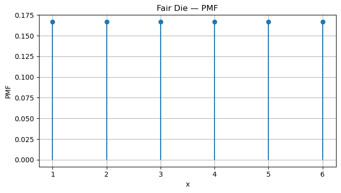
\[\sum_{x} p_X(x) = 1.\]

Example: For a fair die,

\[p_X(x) = \frac{1}{6}, \quad x \in \{1,2,3,4,5,6\}.\]

In RL, the PMF might represent:

the probability of choosing each discrete action under a stochastic policy $\pi(a \mid s)$
the distribution over discrete rewards or terminal states.

Continuous Random Variables — PDF

For continuous random variables, probabilities are defined over intervals via the probability density function (PDF):

\[f_X(x) \ge 0, \quad \int_{-\infty}^{\infty} f_X(x) \, dx = 1.\]

Since single points have zero probability:

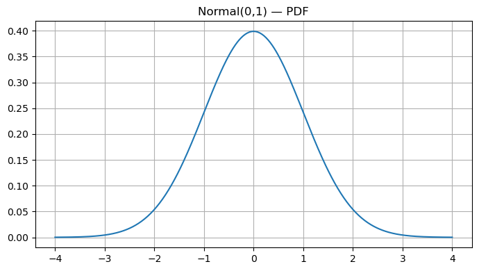
\[\Pr[a \le X \le b] = \int_{a}^{b} f_X(x)\,dx.\]

Example:
If $X \sim \mathcal{N}(0,1)$, then

\[f_X(x) = \frac{1}{\sqrt{2\pi}} e^{-x^2/2}.\]

In RL, PDFs appear when:

policies are continuous (e.g., Gaussian policy $\pi(a \mid s) = \mathcal{N}(\mu(s), \sigma^2(s))$)
environments have continuous state or action spaces**

Cumulative Distribution Function — CDF

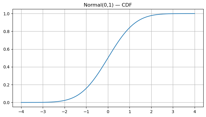
The cumulative distribution function (CDF) gives cumulative probability up to a point:

\[F_X(t) = \Pr[X \le t].\]

For discrete RVs:

\[F_X(t) = \sum_{x \le t} p_X(x),\]

and for continuous ones:

\[F_X(t) = \int_{-\infty}^{t} f_X(x)\,dx.\]

The CDF is always non-decreasing, with $F_X(-\infty)=0$ and $F_X(\infty)=1$. If $X$ is continuous and differentiable, $f_X(x) = \frac{d}{dx}F_X(x)$.

In RL, the CDF helps when:

computing value-at-risk (VaR) or quantile-based objectives (used in distributional RL like C51 or QR-DQN)
analyzing return distributions instead of just expectations

RL Connection

RL Concept	Random Variable Analogy
Reward $R_t$	Sample from a stochastic reward distribution
Return $G_t = \sum \gamma^k R_{t+k}$	Sum of dependent random variables
Policy $\pi(a \mid s)$	PMF/PDF over actions
Exploration noise	Continuous distribution (e.g., Gaussian) added to deterministic policy
Distributional RL	Models the full return CDF, not just the mean value function

Understanding PMFs, PDFs, and CDFs lays the foundation for policy learning, return estimation, and probabilistic reasoning in reinforcement learning.

Code:

# Discrete example: PMF of a fair die
vals = np.arange(1, 7)
pmf = np.full_like(vals, 1/6, dtype=float)

plt.figure()
plt.stem(vals, pmf, basefmt=" ", markerfmt="o", linefmt="-")
plt.xlabel("x")
plt.ylabel("PMF")
plt.title("Fair Die — PMF")
plt.tight_layout()
plt.show()

# Continuous example: PDF & CDF of Normal(0,1)
from math import erf

def norm_pdf(x, mu=0.0, sigma=1.0):
    return (1.0 / (sigma * math.sqrt(2 * math.pi))) * np.exp(-0.5 * ((x - mu) / sigma) ** 2)

def norm_cdf(x, mu=0.0, sigma=1.0):
    from scipy.special import erf
    z = (x - mu) / (sigma * math.sqrt(2))
    return 0.5 * (1 + erf(z))

x = np.linspace(-4, 4, 400)

plt.figure()
plt.plot(x, norm_pdf(x))
plt.title("Normal(0,1) — PDF")
plt.tight_layout()
plt.show()

plt.figure()
plt.plot(x, norm_cdf(x))
plt.title("Normal(0,1) — CDF")
plt.tight_layout()
plt.show()

png

2. Expectation & Variance

Intuition

The expectation (or expected value) and variance are the two most fundamental numerical summaries of a random variable.
They describe:

Expectation → the average or central tendency of the distribution.
Variance → how spread out or uncertain the outcomes are around that average.

In reinforcement learning (RL), these concepts directly underlie:

Expected return (what we maximize)
Reward variance (which affects stability and exploration)
Policy gradient variance (a key challenge in training)

Expectation — “the long-run average”

The expectation of a random variable $X$ represents the average value we would obtain if we repeated the random process infinitely many times.

For a discrete random variable:

\[\mathbb{E}[X] = \sum_x x \, p(x)\]

For a continuous random variable:

\[\mathbb{E}[X] = \int_{-\infty}^{\infty} x \, f(x)\, dx\]

Think of expectation as a “weighted average,” where each possible value of $X$ is weighted by its probability of occurring.

Example (Bernoulli $p$):
For $ X \in {0, 1} $ with $ \Pr[X=1]=p $,

\[\mathbb{E}[X] = 0 \cdot (1-p) + 1 \cdot p = p\]

So the expected number of successes in one Bernoulli trial equals the probability of success itself.

Variance — “measuring uncertainty”

The variance measures how far outcomes tend to deviate from their mean. It is defined as:

\[\mathrm{Var}(X) = \mathbb{E}\big[(X - \mu)^2\big] = \mathbb{E}[X^2] - (\mathbb{E}[X])^2\]

where $ \mu = \mathbb{E}[X] $.

The standard deviation is simply the square root of the variance:

\[\sigma_X = \sqrt{\mathrm{Var}(X)}.\]

A larger variance means outcomes are more unpredictable — critical in RL, where high variance in returns or gradients can destabilize learning.

Example (Bernoulli $p$):

\[\mathrm{Var}(X) = p(1 - p)\]

When $p = 0.5$, uncertainty is highest (max variance); when $p$ is near 0 or 1, variance is small — outcomes are predictable.

Linearity of Expectation

A beautiful property: expectation is always linear, even if random variables are dependent.

For constants $a,b$:

\[\mathbb{E}[aX + b] = a\,\mathbb{E}[X] + b\]

and for multiple random variables:

\[\mathbb{E}\Big[\sum_i X_i\Big] = \sum_i \mathbb{E}[X_i]\]

This property is used throughout RL, for example when analyzing expected returns or when computing value functions from reward sequences.

RL Connections

Concept	Description	Mathematical Tie-In
Expected Return	RL agents aim to maximize expected cumulative reward.	$ J(\pi) = \mathbb{E}_{\pi}\big[\sum_{t=0}^{\infty} \gamma^t R_t\big] $
Policy Gradient	Gradients of expected return rely on linearity of expectation.	$ \nabla_\theta J(\pi_\theta) = \mathbb{E}_{\pi}[\nabla_\theta \log \pi_\theta(a\|s) G_t] $
Variance Reduction	High gradient variance slows learning; baselines and entropy regularization reduce it.	$ \mathrm{Var}[G_t] \downarrow \Rightarrow \text{more stable updates} $
Risk-Sensitive RL	Some tasks care not only about the mean but also about reward variability.	$ \text{Optimize } \mathbb{E}[G_t] - \lambda \mathrm{Var}[G_t] $

Code:

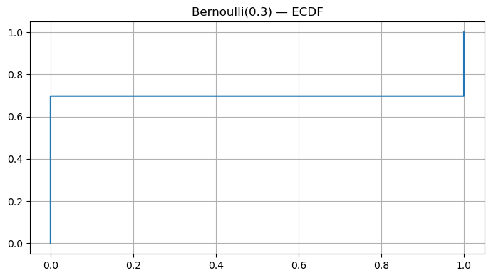
p = 0.3
samples = rng.binomial(n=1, p=p, size=50_000)
est_mean, est_var = samples.mean(), samples.var(ddof=0)
theory_mean, theory_var = p, p*(1-p)
print({"est_mean": round(est_mean,4), "theory_mean": theory_mean})
print({"est_var": round(est_var,4), "theory_var": theory_var})

# ECDF of Bernoulli
x_ecdf, y_ecdf = ecdf(samples)
plt.figure()
plt.step(x_ecdf, y_ecdf, where='post')
plt.title("Bernoulli(0.3) — ECDF")
plt.tight_layout(); plt.show()

Output:

{'est_mean': np.float64(0.3023), 'theory_mean': 0.3}
{'est_var': np.float64(0.2109), 'theory_var': 0.21}

png

3. Canonical Distributions

Probability distributions describe how uncertainty is structured — how likely different outcomes are. In Reinforcement Learning (RL), nearly every component (rewards, actions, transitions) involves random variables. Understanding these canonical distributions gives the mathematical foundation for modeling, exploration, and inference.

1. Bernoulli Distribution — “One Shot, Two Outcomes”

Represents a single binary event — success (1) or failure (0).

\[X \sim \text{Bernoulli}(p), \quad p_X(x) = \begin{cases} p & x = 1 \\ 1-p & x = 0 \end{cases}\]

Expectation: $\mathbb{E}[X] = p$
Variance: $\mathrm{Var}(X) = p(1-p)$

RL Connection:

Represents stochastic binary actions (e.g., “jump” vs “don’t jump”).
Used in ε-greedy exploration: pick a random action with prob. $\varepsilon$.
Models binary rewards (win/loss, success/failure).

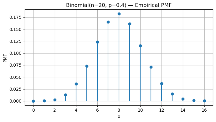
2. Binomial Distribution — “Many Independent Bernoulli Trials”

Represents the number of successes in $n$ independent Bernoulli trials.

\[X \sim \text{Binomial}(n,p), \quad p_X(k) = \binom{n}{k} p^k (1-p)^{n-k}\]

Expectation: $\mathbb{E}[X] = np$
Variance: $\mathrm{Var}(X) = np(1-p)$

RL Connection:

Used to model success counts during episodes or rollouts (e.g., number of wins).
Appears when evaluating Monte Carlo estimates over multiple trials.

3. Geometric Distribution — “How Long Until Success?”

Represents the number of trials until the first success.

\[X \sim \text{Geometric}(p), \quad p_X(k) = (1-p)^{k-1}p, \quad k = 1,2,\dots\]

Expectation: $\mathbb{E}[X] = \frac{1}{p}$
Variance: $\mathrm{Var}(X) = \frac{1-p}{p^2}$

RL Connection:

Models waiting time for a successful episode or goal.
The memoryless property reflects many RL processes where only the current state matters — no dependence on the past.

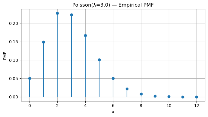
4. Poisson Distribution — “Counting Rare Events”

Represents the number of events occurring in a fixed time or space interval.

\[X \sim \text{Poisson}(\lambda), \quad p_X(k) = e^{-\lambda} \frac{\lambda^k}{k!}, \quad k=0,1,2,\dots\]

Expectation: $\mathbb{E}[X] = \lambda$
Variance: $\mathrm{Var}(X) = \lambda$

RL Connection:

Models event arrivals (e.g., rare rewards or resets).
Useful in environment modeling where transitions or rewards are asynchronous or stochastic in time.

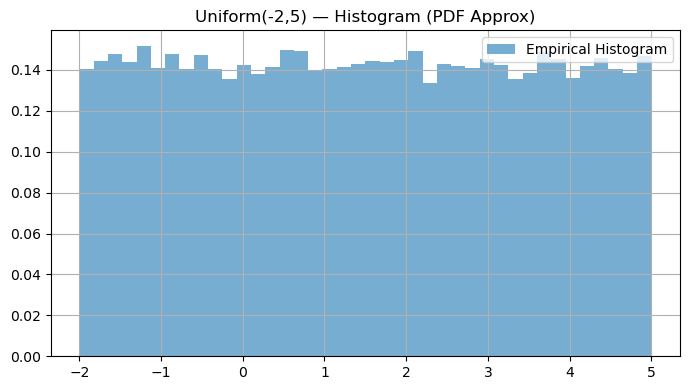
5. Uniform Distribution — “All Outcomes Equally Likely”

Every outcome in an interval $[a,b]$ has equal probability.

\[X \sim \text{Uniform}[a,b], \quad f_X(x) = \begin{cases} \frac{1}{b-a}, & a \le x \le b \\ 0, & \text{otherwise} \end{cases}\]

Expectation: $\mathbb{E}[X] = \frac{a+b}{2}$
Variance: $\mathrm{Var}(X) = \frac{(b-a)^2}{12}$

RL Connection:

Common for random initialization of parameters, actions, or states.
Uniform exploration (before learning begins).

6. Normal (Gaussian) Distribution — “Central Limit Behavior”

Describes many natural random processes due to the Central Limit Theorem (CLT).

\[X \sim \mathcal{N}(\mu, \sigma^2), \quad f_X(x) = \frac{1}{\sqrt{2\pi\sigma^2}} \exp\!\left(-\frac{(x-\mu)^2}{2\sigma^2}\right)\]

Expectation: $\mathbb{E}[X] = \mu$
Variance: $\mathrm{Var}(X) = \sigma^2$

RL Connection:

Fundamental in Gaussian policies for continuous action spaces.
Used in policy gradient methods (e.g., PPO, DDPG) to model $\pi(a \mid s) = \mathcal{N}(\mu_\theta(s), \sigma^2_\theta(s))$.
Appears in noise processes for exploration (Ornstein–Uhlenbeck, Gaussian).

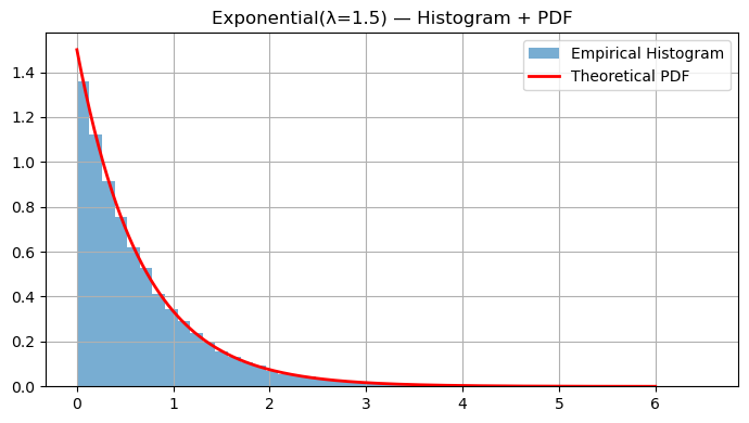
7. Exponential Distribution — “Waiting Time Between Poisson Events”

Represents the time between events in a Poisson process.

\[X \sim \text{Exponential}(\lambda), \quad f_X(x) = \lambda e^{-\lambda x}, \quad x \ge 0\]

Expectation: $\mathbb{E}[X] = \frac{1}{\lambda}$
Variance: $\mathrm{Var}(X) = \frac{1}{\lambda^2}$

RL Connection:

Models waiting time until next event/reward.
Appears in continuous-time RL or semi-Markov decision processes (SMDPs), where actions have variable durations.

Code:

# Binomial(n,p): empirical PMF
n, p = 20, 0.4
binom_samples = rng.binomial(n=n, p=p, size=50_000)
counts = Counter(binom_samples)
xs = np.array(sorted(counts.keys()))
ys = np.array([counts[k] for k in xs]) / len(binom_samples)

plt.figure()
plt.stem(xs, ys, basefmt=" ", markerfmt="o", linefmt="-")
plt.xlabel("x")
plt.ylabel("PMF")
plt.title(f"Binomial(n={n}, p={p}) — Empirical PMF")
plt.tight_layout()
plt.show()

# Poisson(lambda): empirical PMF
lam = 3.0
pois = rng.poisson(lam=lam, size=50_000)
counts = Counter(pois)
xs = np.array(sorted(counts.keys()))
ys = np.array([counts[k] for k in xs]) / len(pois)

plt.figure()
plt.stem(xs, ys, basefmt=" ", markerfmt="o", linefmt="-")
plt.xlabel("x")
plt.ylabel("PMF")
plt.title(f"Poisson(λ={lam}) — Empirical PMF")
plt.tight_layout()
plt.show()

# Uniform(a,b) and Exponential(lambda)
def hist_with_pdf(samples, bins=50, pdf=None, xpdf=None, title=None):
    plt.figure()
    plt.hist(samples, bins=bins, density=True, alpha=0.6, label="Empirical Histogram")
    if pdf is not None and xpdf is not None:
        plt.plot(xpdf, pdf, "r-", lw=2, label="Theoretical PDF")
    plt.title(title)
    plt.legend()
    plt.tight_layout()
    plt.show()

# Uniform
a, b = -2, 5
U = rng.uniform(a, b, size=50_000)
hist_with_pdf(U, bins=40, title="Uniform(-2,5) — Histogram (PDF Approx)")

# Exponential
lam = 1.5
Exp = rng.exponential(1/lam, size=50_000)
xpdf = np.linspace(0, 6, 400)
exp_pdf = lam * np.exp(-lam * xpdf)
hist_with_pdf(Exp, bins=50, pdf=exp_pdf, xpdf=xpdf, title="Exponential(λ=1.5) — Histogram + PDF")

png

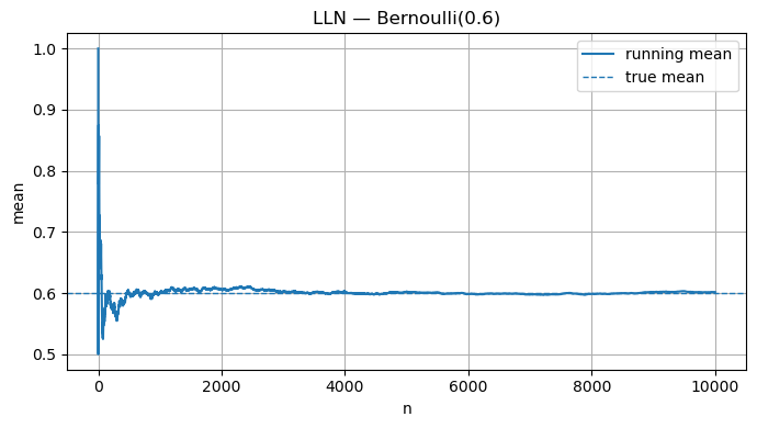
4. Law of Large Numbers (LLN)

The Law of Large Numbers (LLN) is one of the cornerstones of probability theory — and it directly connects to how reinforcement learning (RL) agents estimate returns and values from experience.

Intuition

Suppose we repeat a random experiment many times, each time obtaining an outcome $X_i$. The sample mean after $n$ trials is:

\[\bar{X}_n = \frac{1}{n}\sum_{i=1}^n X_i\]

The Law of Large Numbers states that as the number of samples grows, the sample mean converges to the true expected value $\mu = \mathbb{E}[X]$:

\[\lim_{n \to \infty} \bar{X}_n = \mu\]

Formally, in probability (weak LLN):

\[\forall \varepsilon > 0, \quad \Pr\big(|\bar{X}_n - \mu| > \varepsilon\big) \to 0 \text{ as } n \to \infty.\]

If convergence happens almost surely (with probability 1), we have the strong LLN.

Intuitive Example

If you flip a fair coin repeatedly, the true mean (probability of heads) is $\mu = 0.5$.

After 10 flips, your sample mean might be 0.4 or 0.7.
After 1000 flips, it will almost surely be close to 0.5.

As $n$ increases, the sample mean becomes more stable and less noisy, illustrating that randomness “averages out” in the long run.

Mathematical Insight

The variance of the sample mean decreases with $n$:

\[\mathrm{Var}[\bar{X}_n] = \frac{\sigma^2}{n},\]

so the spread of sample means around the true mean $\mu$ gets smaller as you collect more data.

This property underlies statistical consistency — empirical estimates become accurate as data accumulates.

RL Connection

The Law of Large Numbers explains why experience-based learning works in reinforcement learning.

RL Concept	LLN Interpretation
Monte Carlo value estimation	Averaging many episode returns $G_t$ approximates $ V(s) = \mathbb{E}_\pi[G_t \mid s_t = s] $.
Q-learning targets	The empirical mean of temporal-difference (TD) targets converges to the true expected value.
Policy gradient estimates	Gradient estimates improve as you average over many sampled trajectories.
Exploration and variance	More data reduces stochasticity in policy/value updates, leading to stable learning.

Essentially, RL algorithms rely on LLN to justify learning from finite samples:

as the number of episodes → ∞, empirical estimates converge to their theoretical expectations.

Code:

p = 0.6
N = 10_000
bern = rng.binomial(1, p, size=N)
running_mean = np.cumsum(bern) / (np.arange(N) + 1)

plt.figure()
plt.plot(running_mean, label="running mean")
plt.axhline(p, linestyle='--', linewidth=1, label="true mean")
plt.xlabel("n"); plt.ylabel("mean"); plt.title("LLN — Bernoulli(0.6)")
plt.legend(); plt.tight_layout(); plt.show()

png

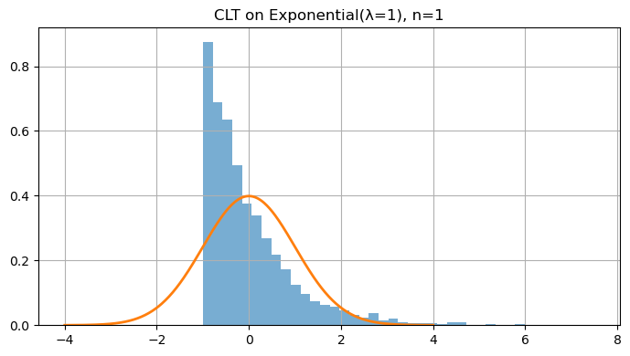
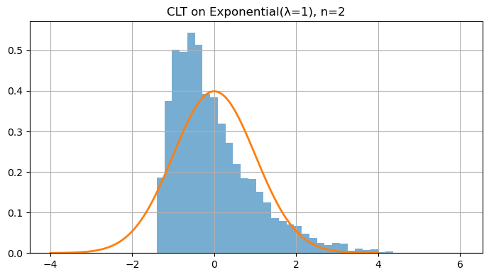
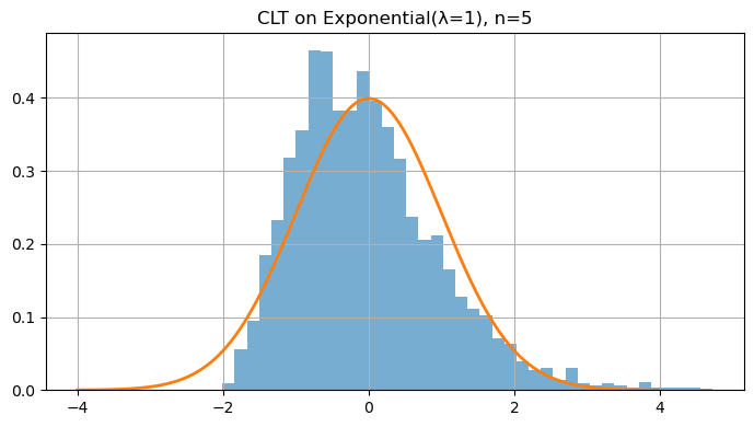
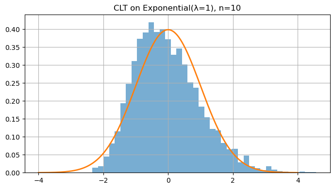
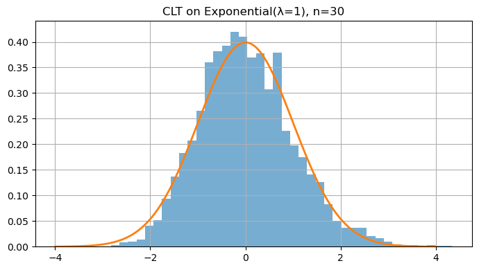
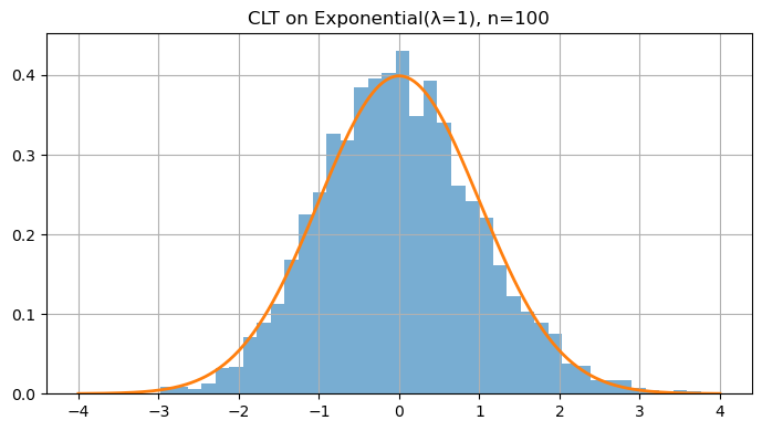
5. Central Limit Theorem (CLT)

The Central Limit Theorem (CLT) is one of the most powerful ideas in probability and statistics. It tells us that averages of random variables tend to follow a Normal (Gaussian) distribution, no matter what the underlying distribution is — provided we have enough independent samples.

Intuition

Let $X_1, X_2, \dots, X_n$ be independent and identically distributed (IID) random variables, each with:

Mean $\mu = \mathbb{E}[X_i]$
Variance $\sigma^2 = \mathrm{Var}(X_i) < \infty$

Then, the standardized sample mean

\[Z_n = \frac{\bar{X}_n - \mu}{\sigma / \sqrt{n}}\]

converges in distribution to the standard normal:

\[Z_n \xrightarrow{d} \mathcal{N}(0,1) \quad \text{as } n \to \infty.\]

In words:

Even if the original data $X_i$ are not normally distributed (e.g., exponential, uniform, or Bernoulli), the distribution of their average $\bar{X}_n$ becomes approximately normal for large $n$.

Why It Matters

This theorem explains why the Normal distribution is everywhere — it emerges naturally as the limit of sums or averages of random variables.

The larger the number of samples $n$, the closer the sample mean’s distribution looks to a bell curve, regardless of the parent distribution.

Mathematically:

$\Pr\left( \frac{\bar{X}_n - \mu}{\sigma/\sqrt{n}} \le z \right) \approx \Phi(z),$ where $\Phi(z)$ is the CDF of $\mathcal{N}(0,1)$.

RL Connection

The CLT provides the theoretical foundation for stability in reinforcement learning:

RL Concept	CLT Interpretation
Monte Carlo return estimates	Averages of episode returns approximate a Normal distribution as sample count increases.
Policy gradient estimation	The stochastic gradient noise becomes approximately Gaussian — enabling the use of variance reduction and adaptive learning-rate methods.
Bootstrapping and TD updates	Aggregated target errors tend toward Gaussianity, improving predictability of learning dynamics.
Confidence intervals for evaluation	Approximate Normality allows for error bars and uncertainty quantification of value estimates.

In short:

The CLT justifies why empirical averages in RL can be treated as normally distributed noise — enabling efficient optimization, statistical inference, and uncertainty modeling.

Code:

def clt_demo(dist_sampler, n, trials=4000):
    means = []
    for _ in range(trials):
        x = dist_sampler(n)
        means.append(np.mean(x))
    return np.array(means)

# Skewed distribution: Exponential(λ=1)
lam = 1.0
def samp_exp(n): return rng.exponential(1/lam, size=n)

for n in [1, 2, 5, 10, 30, 100]:
    means = clt_demo(samp_exp, n=n, trials=4000)
    mu, var = 1/lam, 1/(lam**2)
    z = (means - mu) / math.sqrt(var/n)  # standardize
    plt.figure()
    plt.hist(z, bins=40, density=True, alpha=0.6)
    x = np.linspace(-4, 4, 400)
    plt.plot(x, (1/np.sqrt(2*np.pi))*np.exp(-x**2/2), linewidth=2)
    plt.title(f"CLT on Exponential(λ=1), n={n}")
    plt.tight_layout(); plt.show()

png

6. Joint & Conditional Probability; Independence; Covariance & Correlation

Reinforcement learning operates in stochastic environments — where states, actions, and rewards are random variables. Understanding joint, conditional, and marginal probabilities is therefore essential for reasoning about uncertainty and dependencies between variables.

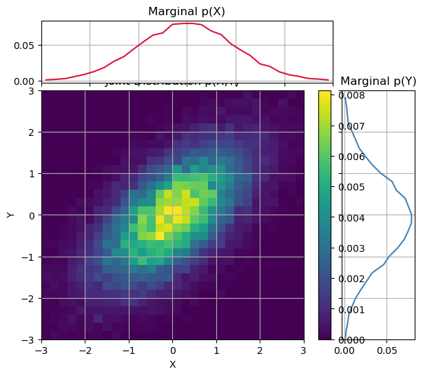
Joint & Marginal Distributions

When we have two random variables $X$ and $Y$, their joint distribution describes the probability of both occurring together:

\[p_{X,Y}(x,y) = \Pr[X = x, Y = y]\]

For continuous variables, we write the joint PDF $f_{X,Y}(x,y)$.

From the joint distribution, we can derive the marginal distributions:

\[p_X(x) = \sum_y p_{X,Y}(x,y), \quad p_Y(y) = \sum_x p_{X,Y}(x,y)\]

or, in the continuous case,

\[f_X(x) = \int_{-\infty}^\infty f_{X,Y}(x,y)\,dy.\]

Conditional Probability

The conditional probability of $Y$ given $X = x$ is:

\[p_{Y \mid X}(y \mid x) = \frac{p_{X,Y}(x,y)}{p_X(x)}.\]

It represents how knowing $X$ changes our belief about $Y$.

For continuous variables, the same relationship holds with PDFs:

\[f_{Y \mid X}(y \mid x) = \frac{f_{X,Y}(x,y)}{f_X(x)}.\]

Independence

Two random variables $X$ and $Y$ are independent if knowledge of one gives no information about the other:

\[X \perp Y \quad \Longleftrightarrow \quad p_{X,Y}(x,y) = p_X(x)p_Y(y)\]

or equivalently, $p_{Y \mid X}(y \mid x) = p_Y(y)$.

This idea of independence is central to simplifying models — in RL, we often assume independence between samples (episodes, transitions) to enable tractable learning.

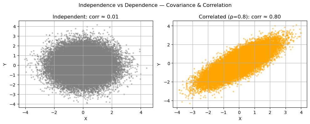
Covariance & Correlation

Covariance measures how two random variables vary together:

\[\mathrm{Cov}(X,Y) = \mathbb{E}[(X - \mu_X)(Y - \mu_Y)].\]

If $X$ and $Y$ increase together, covariance is positive; if one increases while the other decreases, it’s negative. However, covariance depends on scale.

The correlation coefficient $\rho(X,Y)$ standardizes it:

\[\rho(X,Y) = \frac{\mathrm{Cov}(X,Y)}{\sigma_X \sigma_Y}, \quad \rho \in [-1, 1].\]

$\rho = 1$: perfectly positively correlated
$\rho = -1$: perfectly negatively correlated
$\rho = 0$: uncorrelated (not necessarily independent)

RL Connection

Joint and conditional probability form the mathematical backbone of RL:

RL Concept	Probabilistic View
Environment dynamics	$p(s_{t+1}, r_t \mid s_t, a_t)$: joint distribution of next state and reward
Transition model	Marginal over rewards: $p(s_{t+1} \mid s_t, a_t) = \sum_{r_t} p(s_{t+1}, r_t \mid s_t, a_t)$
Policy stochasticity	$\pi(a \mid s) = p(A_t = a \mid S_t = s)$: a conditional distribution over actions
Credit assignment	Correlation between actions $A_t$ and future returns $G_t$ drives policy improvement
Exploration–exploitation trade-off	Managing dependence between visited states and action probabilities

These concepts explain why RL is probabilistic at its core — from policy sampling to estimating expected returns.

Code:

# Joint, Marginal, and Conditional Probability Example
rng = np.random.default_rng(0)

# Bivariate Normal with correlation ρ = 0.6
rho = 0.6
cov = np.array([[1.0, rho], [rho, 1.0]])
XY = rng.multivariate_normal([0, 0], cov, size=20_000)
X, Y = XY[:, 0], XY[:, 1]

# Empirical joint distribution via 2D histogram
nbins = 30
x_edges = np.linspace(-3, 3, nbins + 1)
y_edges = np.linspace(-3, 3, nbins + 1)
H, _, _ = np.histogram2d(X, Y, bins=[x_edges, y_edges])
H /= H.sum()  # normalize → joint pmf/pdf estimate

# Marginals
pX = H.sum(axis=1, keepdims=True)
pY = H.sum(axis=0, keepdims=True)

# Conditional p(Y|X) for one X-bin (≈ x=1)
x_centers = 0.5 * (x_edges[1:] + x_edges[:-1])
ix = np.argmin(np.abs(x_centers - 1.0))
cond = H[ix, :] / (pX[ix, 0] + 1e-12)

# --- Joint and Marginals ---
fig = plt.figure(figsize=(7, 6))
gs = fig.add_gridspec(2, 2, width_ratios=[4, 1], height_ratios=[1, 4],
                      wspace=0.05, hspace=0.05)

ax_joint = fig.add_subplot(gs[1, 0])
ax_marg_x = fig.add_subplot(gs[0, 0], sharex=ax_joint)
ax_marg_y = fig.add_subplot(gs[1, 1], sharey=ax_joint)

# Joint (2D heatmap)
im = ax_joint.imshow(H.T, origin='lower',
                     extent=[x_edges[0], x_edges[-1], y_edges[0], y_edges[-1]],
                     aspect='auto', cmap='viridis')
ax_joint.set_xlabel("X"); ax_joint.set_ylabel("Y")
ax_joint.set_title("Joint Distribution p(X,Y)")
fig.colorbar(im, ax=ax_joint, orientation='vertical', fraction=0.05)

# Marginals
ax_marg_x.plot(x_centers, pX, color='crimson')
ax_marg_x.set_title("Marginal p(X)")
ax_marg_y.plot(pY.ravel(), y_edges[:-1], color='steelblue')
ax_marg_y.set_title("Marginal p(Y)")
ax_marg_x.tick_params(axis="x", labelbottom=False)
ax_marg_y.tick_params(axis="y", labelleft=False)
plt.show()

# Independence vs Dependence + Covariance/Correlation
rng = np.random.default_rng(1)

# (a) Independent variables
X_ind = rng.normal(size=50_000)
Y_ind = rng.normal(size=50_000)
cov_ind  = np.cov(X_ind, Y_ind, ddof=0)[0, 1]
corr_ind = np.corrcoef(X_ind, Y_ind)[0, 1]

# (b) Correlated variables (ρ ≈ 0.8)
rho = 0.8
cov = np.array([[1.0, rho], [rho, 1.0]])
XY = rng.multivariate_normal([0, 0], cov, size=50_000)
X_dep, Y_dep = XY[:, 0], XY[:, 1]
cov_dep  = np.cov(X_dep, Y_dep, ddof=0)[0, 1]
corr_dep = np.corrcoef(X_dep, Y_dep)[0, 1]

# --- Visualization 3: Scatter comparison ---
fig, axs = plt.subplots(1, 2, figsize=(10, 4))
axs[0].scatter(X_ind, Y_ind, s=6, alpha=0.4, color='gray')
axs[0].set_title(f"Independent: corr ≈ {corr_ind:.2f}")
axs[0].set_xlabel("X"); axs[0].set_ylabel("Y")

axs[1].scatter(X_dep, Y_dep, s=6, alpha=0.4, color='orange')
axs[1].set_title(f"Correlated (ρ=0.8): corr ≈ {corr_dep:.2f}")
axs[1].set_xlabel("X"); axs[1].set_ylabel("Y")

plt.suptitle("Independence vs Dependence — Covariance & Correlation")
plt.tight_layout()
plt.show()

png

7. Bayes’ Theorem — Diagnostic Testing

Concept

Bayes’ rule allows us to reverse conditional probabilities — updating beliefs about a cause $A$ after observing evidence $B$:

\[\Pr(A \mid B) = \frac{\Pr(B \mid A)\Pr(A)}{\Pr(B \mid A)\Pr(A) + \Pr(B \mid \neg A)\Pr(\neg A)}.\]

It formalizes belief updating — how prior knowledge (before observing data) combines with evidence (likelihood) to form a posterior belief.

Example

Suppose:

Disease prevalence (prior): $\Pr(A) = 0.01$
Test sensitivity: $\Pr(B \mid A) = 0.95$
Test specificity: $\Pr(\neg B \mid \neg A) = 0.95$

Then:

\[\Pr(A \mid B) = \frac{0.95 \times 0.01}{0.95 \times 0.01 + 0.05 \times 0.99} \approx 0.161.\]

Even with a 95% accurate test, if the disease is rare, most positive results are false positives.

RL Connection

Bayesian reasoning appears in many RL and AI settings:

Bayesian RL maintains a belief $p(\text{model parameters} \mid \text{data})$ and updates it as evidence accumulates.
Thompson Sampling uses posteriors for exploration–exploitation balance.
Uncertainty-aware policies use Bayes’ rule to reason about partially observed or stochastic environments.

In short:

Bayes’ theorem provides the mathematical foundation for belief updates and uncertainty modeling in RL.

Code:

prev = 0.01     # P(D)
sens = 0.95     # P(+|D)
spec = 0.95     # P(-|~D) -> so P(+|~D)=1-spec

pD = prev
pNotD = 1 - prev
p_pos_given_D = sens
p_pos_given_notD = 1 - spec

pD_given_pos = (p_pos_given_D*pD) / (p_pos_given_D*pD + p_pos_given_notD*pNotD)
print("Bayes (closed-form):  P(D|+) =", round(pD_given_pos, 4))

# Monte Carlo check
N = 1_000_00
disease = rng.binomial(1, pD, size=N)
pos = np.where(disease==1,
               rng.binomial(1, p_pos_given_D, size=N),
               rng.binomial(1, p_pos_given_notD, size=N))
est = disease[pos==1].mean()
print("Monte Carlo estimate ≈", round(float(est), 4))

Output:

Bayes (closed-form):  P(D|+) = 0.161
Monte Carlo estimate ≈ 0.1617

Key Takeaways

PMF, PDF, CDF — define how probability is distributed (discrete vs continuous).
Expectation & Variance — capture average behavior and uncertainty.
LLN & CLT — averages converge to true means and approximate normality as samples grow.
Joint, Conditional, & Correlation — describe dependencies between random variables.
Bayes’ Theorem — updates beliefs using prior knowledge and new evidence.

Foundations for probability are core to RL’s stochastic policies, rewards, and belief updates.

Next: 01_linear_algebra_calc.ipynb → matrix calculus, gradients, Jacobians, and chain rule with visual intuition.

Concept	Description	Mathematical Tie-In
Expected Return	RL agents aim to maximize expected cumulative reward.	\( J(\pi) = \mathbb{E}_{\pi}\big[\sum_{t=0}^{\infty} \gamma^t R_t\big] \)
Policy Gradient	Gradients of expected return rely on linearity of expectation.	\( \nabla_\theta J(\pi_\theta) = \mathbb{E}_{\pi}[\nabla_\theta \log \pi_\theta(a\|s) G_t] \)
Variance Reduction	High gradient variance slows learning; baselines and entropy regularization reduce it.	\( \mathrm{Var}[G_t] \downarrow \Rightarrow \text{more stable updates} \)
Risk-Sensitive RL	Some tasks care not only about the mean but also about reward variability.	\( \text{Optimize } \mathbb{E}[G_t] - \lambda \mathrm{Var}[G_t] \)