End-to-End Linear Regression Project

California Housing Prices: from raw data → model → mini “deployment”.

Goal:
Build a complete regression pipeline on a real-world dataset:

• Load and inspect a real housing dataset (California census tracts).
• Perform EDA: distributions, correlations, feature–target relationships.
• Do basic preprocessing and train–validation splitting.
• Train and compare several linear models (OLS, Ridge, Lasso).
• Evaluate with MSE / MAE / R², plus visual diagnostics.
• Wrap the best model into a tiny prediction function as a mini “deployment”.

This project glues together ideas from:

• Probability & statistics (noise, variance, metrics)
• Linear algebra & gradient-based optimization
• Basic ML (regression, regularization, model selection)

Code:

import numpy as np
import pandas as pd
import matplotlib.pyplot as plt
import seaborn as sns

from sklearn.datasets import fetch_california_housing
from sklearn.model_selection import train_test_split, cross_val_score
from sklearn.preprocessing import StandardScaler, PolynomialFeatures
from sklearn.pipeline import Pipeline
from sklearn.linear_model import LinearRegression, Ridge, Lasso
from sklearn.metrics import mean_squared_error, mean_absolute_error, r2_score

# Reproducibility
RANDOM_STATE = 42
np.random.seed(RANDOM_STATE)

plt.style.use("seaborn-v0_8-whitegrid")
plt.rcParams["figure.figsize"] = (6.4, 3.8)
plt.rcParams["axes.titlesize"] = 12

1. Dataset & Problem Statement

We’ll use California housing data:

• Each row = a census block group in California.
• Features (per block): median income, house age, average rooms, population, latitude/longitude, etc.
• Target: MedHouseVal — median house value (in $100,000s).

Task:
Given block-level features, predict the median house value.

This is a tabular regression problem, very typical in applied ML.

Code:

# Load into DataFrame
cal = fetch_california_housing(as_frame=True)
df = cal.frame.copy()

print("Shape:", df.shape)
df.head()

Output:

Shape: (20640, 9)

	MedInc	HouseAge	AveRooms	AveBedrms	Population	AveOccup	Latitude	Longitude	MedHouseVal
0	8.3252	41.0	6.984127	1.023810	322.0	2.555556	37.88	-122.23	4.526
1	8.3014	21.0	6.238137	0.971880	2401.0	2.109842	37.86	-122.22	3.585
2	7.2574	52.0	8.288136	1.073446	496.0	2.802260	37.85	-122.24	3.521
3	5.6431	52.0	5.817352	1.073059	558.0	2.547945	37.85	-122.25	3.413
4	3.8462	52.0	6.281853	1.081081	565.0	2.181467	37.85	-122.25	3.422

Code:

df.info()

Output:

<class 'pandas.core.frame.DataFrame'>
RangeIndex: 20640 entries, 0 to 20639
Data columns (total 9 columns):
 #   Column       Non-Null Count  Dtype  
---  ------       --------------  -----  
 0   MedInc       20640 non-null  float64
 1   HouseAge     20640 non-null  float64
 2   AveRooms     20640 non-null  float64
 3   AveBedrms    20640 non-null  float64
 4   Population   20640 non-null  float64
 5   AveOccup     20640 non-null  float64
 6   Latitude     20640 non-null  float64
 7   Longitude    20640 non-null  float64
 8   MedHouseVal  20640 non-null  float64
dtypes: float64(9)
memory usage: 1.4 MB

2. Exploratory Data Analysis (EDA)

Questions we’ll quickly explore:

• What are the ranges and scales of each feature?
• Are there obvious outliers or heavy skew?
• Which features correlate most with house value?
• How does the target distribution look?

This guides preprocessing (e.g., scaling, transforms) and model choice.

Code:

# Descriptive Stats & Target Distribution
df.describe().T

Output:

	count	mean	std	min	25%	50%	75%	max
MedInc	20640.0	3.870671	1.899822	0.499900	2.563400	3.534800	4.743250	15.000100
HouseAge	20640.0	28.639486	12.585558	1.000000	18.000000	29.000000	37.000000	52.000000
AveRooms	20640.0	5.429000	2.474173	0.846154	4.440716	5.229129	6.052381	141.909091
AveBedrms	20640.0	1.096675	0.473911	0.333333	1.006079	1.048780	1.099526	34.066667
Population	20640.0	1425.476744	1132.462122	3.000000	787.000000	1166.000000	1725.000000	35682.000000
AveOccup	20640.0	3.070655	10.386050	0.692308	2.429741	2.818116	3.282261	1243.333333
Latitude	20640.0	35.631861	2.135952	32.540000	33.930000	34.260000	37.710000	41.950000
Longitude	20640.0	-119.569704	2.003532	-124.350000	-121.800000	-118.490000	-118.010000	-114.310000
MedHouseVal	20640.0	2.068558	1.153956	0.149990	1.196000	1.797000	2.647250	5.000010

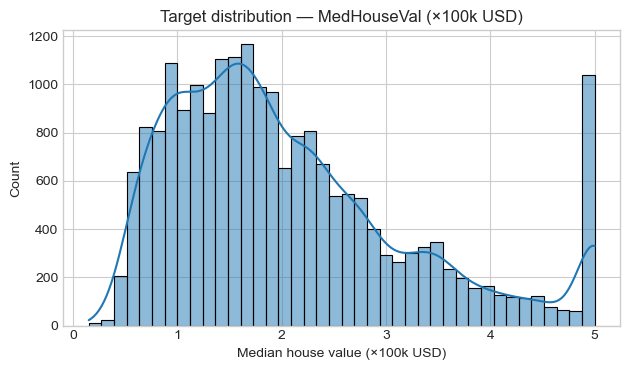
Code:

# Target Histogram
plt.figure()
sns.histplot(df["MedHouseVal"], kde=True, bins=40)
plt.title("Target distribution — MedHouseVal (×100k USD)")
plt.xlabel("Median house value (×100k USD)")
plt.tight_layout()
plt.show()

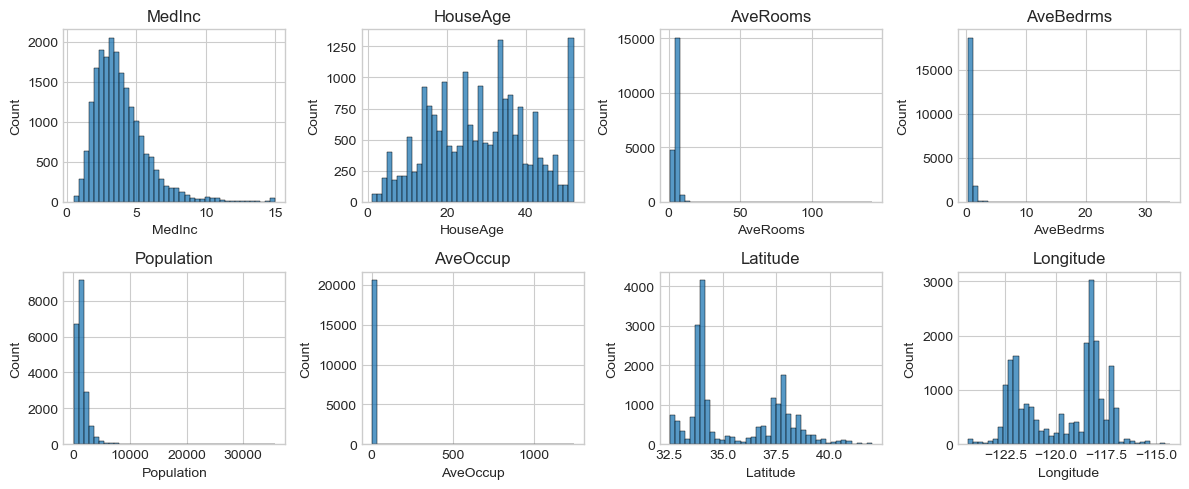
Code:

# Feature Histograms
fig, axes = plt.subplots(2, 4, figsize=(12, 5))
axes = axes.ravel()

for col, ax in zip(df.columns[:-1], axes): # all features except target
    sns.histplot(df[col], bins=40, ax=ax)
    ax.set_title(col)

plt.tight_layout()
plt.show()

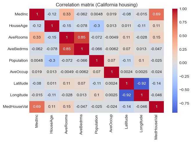
Code:

# Correlation with target
corr = df.corr(numeric_only=True)
corr["MedHouseVal"].sort_values(ascending=False)

Output:

MedHouseVal    1.000000
MedInc         0.688075
AveRooms       0.151948
HouseAge       0.105623
AveOccup      -0.023737
Population    -0.024650
Longitude     -0.045967
AveBedrms     -0.046701
Latitude      -0.144160
Name: MedHouseVal, dtype: float64

Code:

# Correlation Heatmap
plt.figure(figsize=(7, 5))
sns.heatmap(corr, cmap="coolwarm", center=0, annot=True)
plt.title("Correlation matrix (California housing)")
plt.tight_layout()
plt.show()

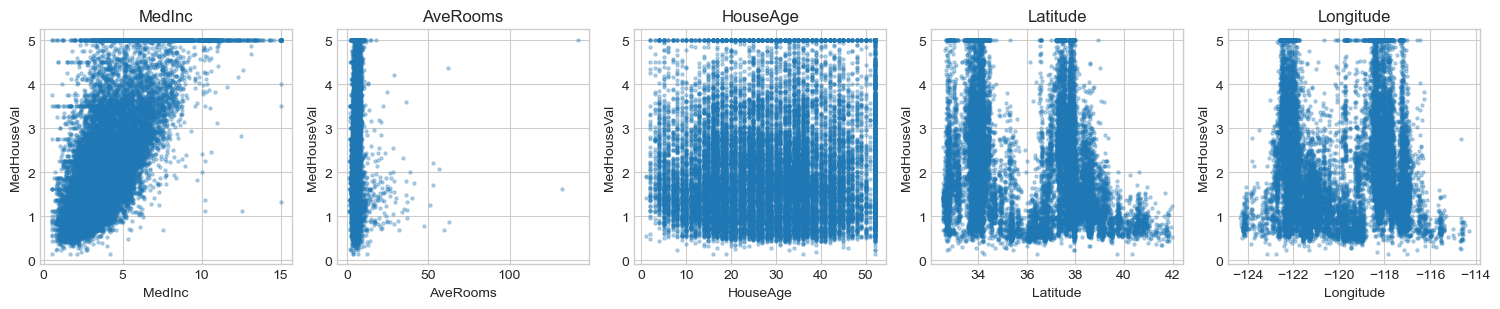
Code:

# Key Feature vs Target Scatter
key_features = ["MedInc", "AveRooms", "HouseAge", "Latitude", "Longitude"]

fig, axes = plt.subplots(1, len(key_features), figsize=(3*len(key_features), 3.2))
for col, ax in zip(key_features, axes):
    ax.scatter(df[col], df["MedHouseVal"], s=5, alpha=0.3)
    ax.set_xlabel(col)
    ax.set_ylabel("MedHouseVal")
    ax.set_title(col)

plt.tight_layout()
plt.show()

3. Train/Validation Split & Baseline

We’ll:

1. Split data into train and test sets (80/20).
2. Build a naive baseline that always predicts the training mean of the target.
3. Compare all later models against this baseline using:

• MSE (Mean Squared Error)
• MAE (Mean Absolute Error)
• R² (coefficient of determination)

Code:

X = df.drop(columns=["MedHouseVal"])
y = df["MedHouseVal"].values

X_train, X_test, y_train, y_test = train_test_split(
    X, y, test_size=0.2, random_state=RANDOM_STATE
)

print("Train shape:", X_train.shape, "Test shape:", X_test.shape)

# Baseline: predict training mean
baseline_pred = np.full_like(y_test, fill_value=y_train.mean(), dtype=float)

def metrics_dict(y_true, y_pred):
    return {
        "MSE": mean_squared_error(y_true, y_pred),
        "MAE": mean_absolute_error(y_true, y_pred),
        "R2":  r2_score(y_true, y_pred),
    }

print("Baseline metrics:", {k: round(v, 3) for k, v in metrics_dict(y_test, baseline_pred).items()})

Output:

Train shape: (16512, 8) Test shape: (4128, 8)
Baseline metrics: {'MSE': 1.311, 'MAE': 0.906, 'R2': -0.0}

4. Preprocessing & Linear Models

We’ll build three linear models wrapped in Pipelines:

1. OLS — LinearRegression with feature standardization.
2. Ridge — L2-regularized regression (controls weight magnitude).
3. Lasso — L1-regularized regression (encourages sparsity).

All preprocessing (here, StandardScaler) happens inside the pipeline to avoid data leakage.

Code:

models = {
    "OLS": Pipeline([
        ("scaler", StandardScaler()),
        ("reg", LinearRegression())
    ]),
    "Ridge(α=1.0)": Pipeline([
        ("scaler", StandardScaler()),
        ("reg", Ridge(alpha=1.0, random_state=RANDOM_STATE))
    ]),
    "Lasso(α=0.001)": Pipeline([
        ("scaler", StandardScaler()),
        ("reg", Lasso(alpha=0.001, random_state=RANDOM_STATE, max_iter=10_000))
    ]),
}

results = []

for name, pipe in models.items():
    pipe.fit(X_train, y_train)
    y_pred = pipe.predict(X_test)
    m = metrics_dict(y_test, y_pred)
    m = {k: round(v, 4) for k, v in m.items()}
    m["Model"] = name
    results.append(m)

results_df = pd.DataFrame(results).set_index("Model").sort_values("R2", ascending=False)
results_df

Output:

	MSE	MAE	R2
Model
Lasso(α=0.001)	0.5545	0.5331	0.5769
OLS	0.5559	0.5332	0.5758
Ridge(α=1.0)	0.5559	0.5332	0.5758

Code:

# Pick Best Model & Diagnostics
best_name = results_df["R2"].idxmax()
best_pipeline = models[best_name]
print(f"Best model by R² on test set: {best_name}")
print(results_df.loc[best_name])

# Predictions from best model
y_pred_best = best_pipeline.predict(X_test)

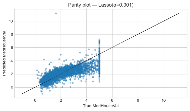
# Parity plot: y_true vs y_pred
plt.figure()
plt.scatter(y_test, y_pred_best, s=10, alpha=0.4)
lims = [min(y_test.min(), y_pred_best.min()), max(y_test.max(), y_pred_best.max())]
plt.plot(lims, lims, "k--", linewidth=1)
plt.title(f"Parity plot — {best_name}")
plt.xlabel("True MedHouseVal")
plt.ylabel("Predicted MedHouseVal")
plt.tight_layout()
plt.show()

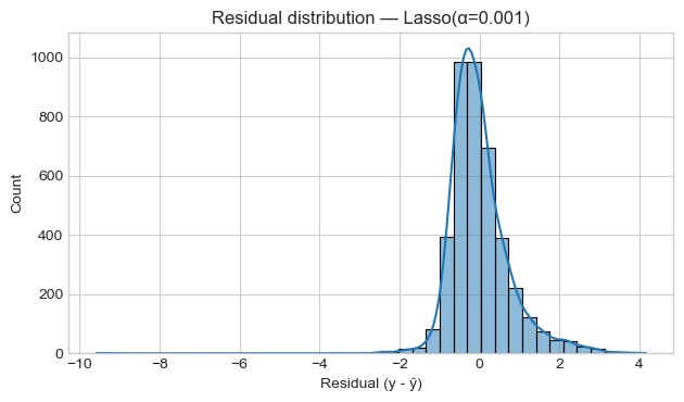
# Residual histogram
residuals = y_test - y_pred_best
plt.figure()
sns.histplot(residuals, bins=40, kde=True)
plt.title(f"Residual distribution — {best_name}")
plt.xlabel("Residual (y - ŷ)")
plt.tight_layout()
plt.show()

Output:

Best model by R² on test set: Lasso(α=0.001)
MSE    0.5545
MAE    0.5331
R2     0.5769
Name: Lasso(α=0.001), dtype: float64

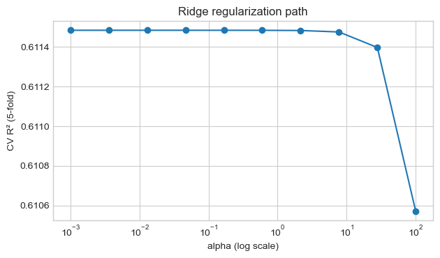
5. Cross-Validation & Hyperparameters (Ridge)

We’ll tune the Ridge regularization strength $\alpha$ using cross-validation on the training set.

• Small $\alpha$: low regularization, risk of overfitting.
• Large $\alpha$: stronger shrinkage, may underfit.

We’ll:

1. Try a grid of $\alpha$ values.
2. Compute 5-fold CV $R^2$ for each.
3. Pick the best $\alpha$ and compare against our previous best model.

Code:

alphas = np.logspace(-3, 2, 10)
cv_scores = []

for a in alphas:
    ridge_pipe = Pipeline([
        ("scaler", StandardScaler()),
        ("reg", Ridge(alpha=a, random_state=RANDOM_STATE))
    ])
    scores = cross_val_score(
        ridge_pipe, X_train, y_train, cv=5,
        scoring="r2", n_jobs=-1
    )
    cv_scores.append(scores.mean())

cv_scores = np.array(cv_scores)

best_alpha = float(alphas[cv_scores.argmax()])
print("Best alpha by CV:", best_alpha)
print("Best mean CV R²:", round(cv_scores.max(), 4))

plt.figure()
plt.semilogx(alphas, cv_scores, marker="o")
plt.xlabel("alpha (log scale)")
plt.ylabel("CV R² (5-fold)")
plt.title("Ridge regularization path")
plt.tight_layout()
plt.show()

Output:

Best alpha by CV: 0.001
Best mean CV R²: 0.6115

Code:

# Train Final Ridge & Compare
ridge_best = Pipeline([
    ("scaler", StandardScaler()),
    ("reg", Ridge(alpha=best_alpha, random_state=RANDOM_STATE))
])
ridge_best.fit(X_train, y_train)
y_pred_ridge_best = ridge_best.predict(X_test)
metrics_ridge_best = {k: round(v, 4) for k, v in metrics_dict(y_test, y_pred_ridge_best).items()}
metrics_ridge_best

Output:

{'MSE': 0.5559, 'MAE': 0.5332, 'R2': 0.5758}

6. Tiny “Deployment” — Prediction Helper

In a real project, the trained pipeline would be:

• Saved to disk (e.g., joblib.dump)
• Loaded inside an API server (FastAPI / Flask) or a batch script
• Used to serve predictions for new data

Here, we’ll simulate a single prediction function:

• Train the chosen model on all data (train + test).
• Define predict_median_value(features_dict) that takes a Python dict and returns a prediction.
• Try it on a realistic example (e.g., middle-income block near the coast).

Code:

deployed_model = ridge_best

# Fit on full dataset
deployed_model.fit(X, y)

feature_names = list(X.columns)
print("Features:", feature_names)

def predict_median_value(features):
    """
    features: dict mapping feature name -> value
              any missing feature will be filled with dataset median.
    returns: predicted median house value in 100k USD.
    """
    x = df[feature_names].median().to_dict() # start from medians
    x.update(features) # override with user values
    x_df = pd.DataFrame([x], columns=feature_names)
    pred = deployed_model.predict(x_df)[0]
    return float(pred)

# Example: relatively high-income coastal block
example_features = {
    "MedInc": 6.0, # median income (~$60k)
    "HouseAge": 20.0,
    "AveRooms": 5.5,
    "AveBedrms": 1.0,
    "Population": 800.0,
    "AveOccup": 2.5,
    "Latitude": 34.0, # SoCal-ish
    "Longitude": -118.3, # near LA
}

pred_val = predict_median_value(example_features)
print(f"Predicted median house value: {pred_val:.3f} × 100k USD (~${pred_val*100_000:,.0f})")

Output:

Features: ['MedInc', 'HouseAge', 'AveRooms', 'AveBedrms', 'Population', 'AveOccup', 'Latitude', 'Longitude']
Predicted median house value: 2.987 × 100k USD (~$298,739)

7. Project Summary & Next Steps

• Loaded and explored the California housing dataset (real census data).
• Performed EDA: distributions, correlations, and key feature–target plots.
• Built a train/test split and a mean baseline for comparison.
• Trained and evaluated OLS, Ridge, and Lasso models with proper scaling.
• Used Ridge + cross-validation to choose a regularization strength.
• Wrapped the final model into a small prediction helper, mimicking deployment.

This project solidifies:

• How linear regression behaves on real, noisy data.
• How to structure an end-to-end ML workflow (EDA → preprocessing → modeling → evaluation → deployment sketch).

Next: Build 10_cnn_image_classification_project.ipynb for a vision-based classification task. Then move on to Phase 1 — Fundamentals (MDPs, Bellman equations, DP, Monte Carlo, TD).