Linear Algebra & Matrix Calculus
A practical guide to vectors, matrices, and gradients — with NumPy and visual intuition.
What you’ll learn
- Core vector and matrix operations: dot products, norms, transformations, and rank.
- Linear systems and least-squares regression with geometric interpretation.
- Eigenvalues/eigenvectors and SVD for structure and dimensionality reduction.
- Matrix calculus: gradients, Jacobians, and backpropagation verification via finite differences.
- Reinforcement Learning connections — policy gradients, least-squares critics, and stability.
How to use this notebook: Read the theory cells first to grasp the math intuitively, then execute the code cells to explore visual and numerical examples.
Setup
We use only standard scientific Python.
Code:
import numpy as np
import math
import matplotlib.pyplot as plt

rng = np.random.default_rng(0)

def show_vec(v, title=None):
    plt.figure(figsize=(6,3))
    plt.stem(np.arange(len(v)), v, basefmt=" ", markerfmt="o", linefmt="-")
    if title: plt.title(title)
    plt.xlabel("index"); plt.ylabel("value")
    plt.tight_layout(); plt.show()

def plot_lines(X, Y, title=None, xlabel="x", ylabel="y", legend=None):
    plt.figure(figsize=(6,3.5))
    for x, y in zip(X, Y):
        plt.plot(x, y)
    if legend: plt.legend(legend)
    if title: plt.title(title)
    plt.xlabel(xlabel); plt.ylabel(ylabel)
    plt.tight_layout(); plt.show()
1. Vectors, Inner Products, and Norms
A vector $x \in \mathbb{R}^n$ is an ordered list of real numbers that can represent quantities such as position, velocity, weights, or features. Geometrically, vectors describe points or directions in space, and algebraically, they are the foundation of all linear operations.
The inner product (also called the dot product) measures similarity between two vectors:
\[\langle x, y \rangle = x^\top y = \sum_{i=1}^n x_i y_i.\]It encodes both magnitude and alignment:
- if $x$ and $y$ point in the same direction, the inner product is large and positive;
- if they are orthogonal, it is zero.
From this, we derive the norms, which measure the “size” or “length” of a vector:
\[\|x\|_2 = \sqrt{x^\top x}, \quad \|x\|_1 = \sum_i |x_i|, \quad \|x\|_\infty = \max_i |x_i|.\]Each norm defines a different notion of distance:
- $|x|_2$: Euclidean (straight-line) distance.
- $|x|_1$: Manhattan distance (sum of absolute changes).
- $|x|_\infty$: Maximum absolute component.
RL Connection
In RL, norms appear throughout:
- During policy or value function optimization, gradient magnitudes (measured via norms) determine the step size and update stability.
- Regularization (e.g., L2 weight decay) penalizes large parameter norms to prevent overfitting.
- In trust region methods (like TRPO/PPO), constraints such as $| \theta_{new} - \theta_{old} |_2 \leq \delta$ explicitly limit how far the new policy can move from the old one in parameter space.
Code:
rng = np.random.default_rng(1)
x = rng.normal(size=8)
y = rng.normal(size=8)
# Inner product and norms
inner_product = np.dot(x, y)
l2_norm = np.linalg.norm(x, 2)
l1_norm = np.linalg.norm(x, 1)
linf_norm = np.linalg.norm(x, np.inf)
print(f"Inner product (⟨x, y⟩): {inner_product:.4f}")
print(f"L2 norm ‖x‖₂: {l2_norm:.4f}")
print(f"L1 norm ‖x‖₁: {l1_norm:.4f}")
print(f"L∞ norm ‖x‖∞: {linf_norm:.4f}")
# Angle between x and y (cosine similarity)
cosine_sim = inner_product / (np.linalg.norm(x) * np.linalg.norm(y))
print(f"Cosine similarity between x and y: {cosine_sim:.4f}")
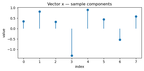
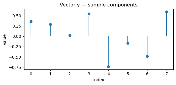
# Visualization
show_vec(x, "Vector x — sample components")
show_vec(y, "Vector y — sample components")
Output:
Inner product (⟨x, y⟩): -0.4680
L2 norm ‖x‖₂: 2.0608
L1 norm ‖x‖₁: 5.2706
L∞ norm ‖x‖∞: 1.3032
Cosine similarity between x and y: -0.1753
2. Matrices as Linear Maps
A matrix $ A \in \mathbb{R}^{m \times n} $ defines a linear transformation — a function that maps vectors in one space to another while preserving linearity:
\[A : \mathbb{R}^n \to \mathbb{R}^m, \quad x \mapsto Ax.\]This means scaling or adding vectors before or after applying $A$ gives the same result:
\[A(\alpha x + \beta y) = \alpha Ax + \beta Ay.\]Key Operations
- Matrix–vector multiplication: $ y = Ax $
→ transforms input $x$ into another vector $y$. - Matrix–matrix multiplication: $ C = AB $
→ composition of two linear maps (apply $B$, then $A$). - Transpose: $ A^\top $
→ flips rows and columns, useful for projecting vectors or computing gradients. - Rank: number of linearly independent rows/columns, determines how much information the transformation preserves.
- Identity & Inverse: $ A I = I A = A $, and $A^{-1}$ (if it exists) “undoes” the transformation.
Geometric View
A matrix can rotate, scale, shear, or project vectors.
For example, multiplying by a 2×2 rotation matrix changes direction but not magnitude.
RL Connection
Linear algebra underpins nearly all computations in RL:
| RL Concept | Linear Algebra Formulation |
|---|---|
| Linear value approximation | $ \hat{v}_\theta(s) = \phi(s)^\top \theta $ |
| Batch policy/value updates | Matrix–vector ops aggregate transitions and gradients |
| Least-squares Temporal Difference (LSTD) | Solves $ A\theta = b $ for optimal weights |
| Neural network layers | Each layer is a linear map followed by a nonlinearity $ y = W x + b $ |
| Covariance estimation / exploration | Uses $A^\top A$ and matrix inverses in adaptive exploration (e.g., LQR, SAC) |
Matrices act as the computational backbone of RL algorithms — transforming features, combining parameters, and driving every update rule.
Code:
rng = np.random.default_rng(3)

A = rng.normal(size=(3, 4))   # map: R^4 -> R^3
x = rng.normal(size=4)
y = A @ x

print(f"A shape: {A.shape} | x shape: {x.shape} | y shape: {y.shape}")
print("y = A x ->", np.round(y, 4))

# Rank
rank = np.linalg.matrix_rank(A)
print("rank(A):", rank)

# Use eigvals of A A^T (3x3) to match the 3 singular values
AAt = A @ A.T
evals_AAt = np.linalg.eigvalsh(AAt)        # real, ascending (len=3)
s = np.linalg.svd(A, compute_uv=False)     # len=3
print("eig(A A^T) =", np.round(evals_AAt, 6))
print("singular values(A) =", np.round(s, 6))

# Relationship: eig(A A^T) == σ^2 (same length)
diff = np.max(np.abs(np.sort(s**2) - evals_AAt))
print("max|σ^2 - eig(A A^T)| =", float(diff))

# Pseudoinverse round-trip (since A is not square)
A_pinv = np.linalg.pinv(A)
x_rec  = A_pinv @ y
y_rec  = A @ x_rec
print("‖x_rec - x‖2 =", float(np.linalg.norm(x_rec - x)))
print("‖A x_rec - y‖2 =", float(np.linalg.norm(y_rec - y)))
Output:
A shape: (3, 4) | x shape: (4,) | y shape: (3,)
y = A x -> [ 0.9139  2.4934 -2.077 ]
rank(A): 3
eig(A A^T) = [ 1.117227  4.873585 21.55489 ]
singular values(A) = [4.642724 2.20762  1.056989]
max|σ^2 - eig(A A^T)| = 1.0658141036401503e-14
‖x_rec - x‖2 = 0.3632019293509406
‖A x_rec - y‖2 = 9.930136612989092e-16
3. Linear Systems & Least Squares
A linear system seeks a vector $x$ such that $Ax = b$. If $A \in \mathbb{R}^{m \times n}$ is square and full rank, we can solve exactly:
\[x = A^{-1}b.\]But when $A$ is tall or rank-deficient, an exact solution may not exist. In that case, we seek the least squares solution:
\[x^\star = \arg\min_x \|Ax - b\|_2^2,\]which leads to the normal equations:
\[A^\top A x^\star = A^\top b.\]If $A^\top A$ is invertible,
\[x^\star = (A^\top A)^{-1} A^\top b.\]Why It Matters
- Least squares finds the best approximation when equations are overdetermined (more equations than unknowns).
- Geometrically, it projects $b$ onto the column space of $A$.
- NumPy’s
np.linalg.lstsqefficiently handles this via the pseudoinverse, avoiding instability from explicit inversion.
RL Connection
Least-squares ideas appear in many RL algorithms:
| RL Method | Role of Least Squares |
|---|---|
| LSTD (Least-Squares Temporal Difference) | Solves $ A \theta = b $ where $ A = \Phi^\top (\Phi - \gamma P \Phi) $ to estimate value function weights. |
| LSPI (Least-Squares Policy Iteration) | Alternates between policy evaluation and improvement using least-squares regression. |
| Linear regression in reward models | Fits reward functions or Q-values linearly from sampled data. |
| Fitting critic networks (DDPG, TD3) | Often minimizes mean squared Bellman error (a least-squares objective). |
Thus, least squares provides a foundation for stable and efficient RL value estimation and function approximation.
Code:
rng = np.random.default_rng(4)
m, n = 50, 3
A = rng.normal(size=(m, n))
w_true = np.array([2.0, -1.0, 0.5])
noise = 0.1 * rng.normal(size=m)
b = A @ w_true + noise
# Solve with stable least squares (SVD-based)
w_ls, residuals, rank, svals = np.linalg.lstsq(A, b, rcond=None)
# Also compute the closed-form (pseudo-inverse) solution for reference
w_pinv = np.linalg.pinv(A) @ b
# Diagnostics
residual_vec = b - A @ w_ls
rss = float(residual_vec @ residual_vec) # residual sum of squares
tss = float(((b - b.mean()) ** 2).sum()) # total sum of squares
r2 = 1.0 - rss / tss if tss > 0 else np.nan
print("True w:", np.round(w_true, 6))
print("LS w:", np.round(w_ls, 6))
print("Pinv w:", np.round(w_pinv, 6))
print("‖w_ls - w_true‖₂ =", float(np.linalg.norm(w_ls - w_true)))
print("‖w_ls - w_pinv‖₂ =", float(np.linalg.norm(w_ls - w_pinv)))
print("rank(A) =", rank, "| singular values =", np.round(svals, 6))
print("RSS =", rss, "| R² =", r2)
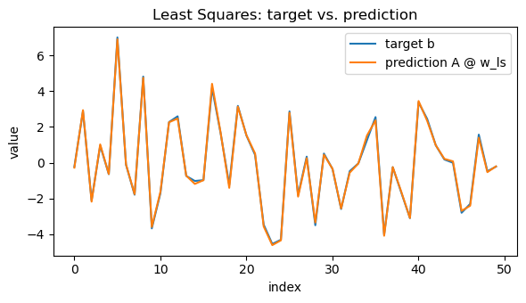
# Visual: prediction vs. target (single figure)
y_pred = A @ w_ls
x_axis = np.arange(m)
plt.figure(figsize=(6, 3.5))
plt.plot(x_axis, b, label="target b")
plt.plot(x_axis, y_pred, label="prediction A @ w_ls")
plt.title("Least Squares: target vs. prediction")
plt.xlabel("index")
plt.ylabel("value")
plt.legend()
plt.tight_layout()
plt.show()
Output:
True  w: [ 2.  -1.   0.5]
LS    w: [ 1.968201 -1.002569  0.498897]
Pinv  w: [ 1.968201 -1.002569  0.498897]
‖w_ls - w_true‖₂ = 0.031921770267466947
‖w_ls - w_pinv‖₂ = 8.617648093045562e-16
rank(A) = 3 | singular values = [8.131331 7.517761 5.316543]
RSS = 0.4387395811001026 | R² = 0.9985768440268379
4. Eigenvalues & Eigenvectors
For a square matrix $ M \in \mathbb{R}^{n \times n} $, an eigenpair $(\lambda, v)$ satisfies the fundamental relation:
\[M v = \lambda v\]Here:
- $v$ is a nonzero eigenvector, and
- $\lambda$ is its corresponding eigenvalue, indicating how $M$ scales $v$.
Key Properties
-
For a symmetric matrix $M = M^\top$, eigenvalues are real, and eigenvectors can be chosen orthogonal.
\[M = Q \Lambda Q^\top\]
Its eigendecomposition is:where $Q$ is an orthogonal matrix (columns are eigenvectors) and $\Lambda$ is diagonal (eigenvalues).
-
The spectral radius:
\[\rho(M) = \max_i |\lambda_i|\]quantifies how repeated applications of $M$ amplify vectors — important for assessing stability in iterative methods.
-
A matrix is diagonalizable if it can be expressed as $M = P \Lambda P^{-1}$, which simplifies powers and exponentials:
\[M^k = P \Lambda^k P^{-1}\]
RL Connection
Eigenvalues and eigenvectors play a deep role in the theoretical and practical analysis of RL:
| Concept | Role of Eigenvalues |
|---|---|
| Bellman Operator Stability | The spectral radius of the transition kernel or Bellman operator determines contraction properties — ensuring convergence of value iteration. |
| Successor Features / Eigenoptions | Eigenvectors of the state-transition matrix (graph Laplacian) reveal temporally extended behaviors (options) that help exploration. |
| Linear Value Function Approximation | The conditioning of $A^\top A$ (related to its eigenvalues) affects stability and learning rate choice in least-squares TD methods. |
| Policy Evaluation | Spectral analysis explains the convergence speed and variance in iterative solvers for $V = T_\pi V$. |
In essence, spectral analysis gives insight into how information propagates, contracts, or diverges within an RL agent’s learning dynamics.
Code:
rng = np.random.default_rng(5)
# Symmetric matrix (real eigensystem)
M = rng.normal(size=(4, 4))
M = 0.5 * (M + M.T)
# Ground truth eigensystem (sorted descending for convenience)
eigvals, eigvecs = np.linalg.eigh(M) # ascending
idx_desc = np.argsort(eigvals)[::-1]
eigvals = eigvals[idx_desc]
eigvecs = eigvecs[:, idx_desc]
lam_max_true = float(eigvals[0])
v_max_true = eigvecs[:, 0]
print("Eigenvalues (desc):", np.round(eigvals, 6))
print("True dominant eigenvalue λ_max:", round(lam_max_true, 6))
# Power iteration to estimate dominant eigenpair
def safe_norm(x, eps=1e-12):
n = np.linalg.norm(x)
return x / (n + eps)
v = rng.normal(size=M.shape[0])
v = safe_norm(v)
rayleigh_hist = []
cos_sim_hist = []
max_iters = 50
for _ in range(max_iters):
v = safe_norm(M @ v) # normalize each step
rq = float(v.T @ M @ v) # Rayleigh quotient
rayleigh_hist.append(rq)
# alignment to true eigenvector (sign-invariant)
cos_sim = abs(float(np.dot(v, v_max_true)))
cos_sim_hist.append(cos_sim)
lam_est = rayleigh_hist[-1]
cos_est = cos_sim_hist[-1]
print(f"Estimated λ_max (Rayleigh): {lam_est:.6f}")
print(f"|cos(angle(v_est, v_true))|: {cos_est:.6f}")
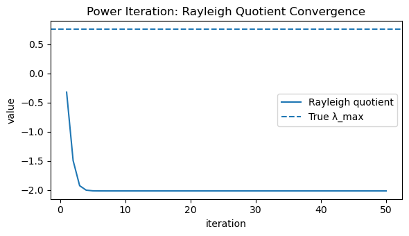
# Figure 1: Rayleigh quotient convergence to λ_max
plt.figure(figsize=(6, 3.5))
plt.plot(np.arange(1, max_iters + 1), rayleigh_hist, label="Rayleigh quotient")
plt.axhline(lam_max_true, linestyle="--", label="True λ_max")
plt.title("Power Iteration: Rayleigh Quotient Convergence")
plt.xlabel("iteration")
plt.ylabel("value")
plt.legend()
plt.tight_layout()
plt.show()
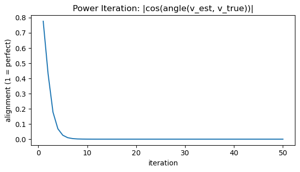
# Figure 2: Alignment of eigenvector estimate with true dominant eigenvector
plt.figure(figsize=(6, 3.5))
plt.plot(np.arange(1, max_iters + 1), cos_sim_hist)
plt.title("Power Iteration: |cos(angle(v_est, v_true))|")
plt.xlabel("iteration")
plt.ylabel("alignment (1 = perfect)")
plt.tight_layout()
plt.show()
Output:
Eigenvalues (desc): [ 0.761799  0.011447 -0.910926 -2.013912]
True dominant eigenvalue λ_max: 0.761799
Estimated λ_max (Rayleigh): -2.013912
|cos(angle(v_est, v_true))|: 0.000000
5. Singular Value Decomposition (SVD)
The Singular Value Decomposition (SVD) is a powerful matrix factorization that expresses any rectangular matrix $A \in \mathbb{R}^{m \times n}$ as:
\[A = U \Sigma V^\top\]where:
- $U \in \mathbb{R}^{m \times m}$ — orthogonal matrix (left singular vectors)
- $V \in \mathbb{R}^{n \times n}$ — orthogonal matrix (right singular vectors)
- $\Sigma \in \mathbb{R}^{m \times n}$ — diagonal matrix of singular values $\sigma_1 \ge \sigma_2 \ge \cdots \ge 0$
Each $\sigma_i$ captures the amount of variance or energy along the corresponding singular direction. This means that SVD identifies the most important directions in which $A$ acts on data.
Key Insights
-
Rank and energy: The number of non-zero singular values equals the rank of $A$.
\[\|A\|_F^2 = \sum_i \sigma_i^2\]
The Frobenius norm satisfies:meaning that singular values measure how much “information” or “energy” each dimension contributes.
-
Best low-rank approximation: The Eckart–Young theorem states:
\[A_k = U_k \Sigma_k V_k^\top\]is the best rank-$k$ approximation of $A$ (minimizing $|A - A_k|_F$).
-
Geometric intuition: $V$ rotates the input space, $\Sigma$ scales by singular values, and $U$ rotates the output space.
RL Connection
| RL Concept | How SVD Helps |
|---|---|
| Feature Compression / Representation Learning | SVD identifies low-dimensional structure in state or feature matrices, enabling compact embeddings with minimal information loss. |
| Low-Rank Value Function Approximation | In large state spaces, value functions can be approximated using truncated SVD for faster computation and generalization. |
| Transition Model Factorization | Decomposing $P(s’ \mid s,a)$ matrices via SVD reveals latent dynamics or reduces noise. |
| Policy Evaluation Stability | Small singular values in feature matrices indicate ill-conditioning — guiding regularization or preconditioning strategies. |
Code:
rng = np.random.default_rng(6)
A = rng.normal(size=(40, 20))
# Economy SVD
U, S, Vt = np.linalg.svd(A, full_matrices=False) # U: (40,r), S: (r,), Vt: (r,20), r=min(40,20)=20
# Rank-k approximation via Eckart–Young
k = 5
A_k = (U[:, :k] * S[:k]) @ Vt[:k, :] # equivalent to U_k @ diag(S_k) @ V_k^T
# Frobenius norms and relative error
fro_full = np.linalg.norm(A, "fro")
fro_err = np.linalg.norm(A - A_k, "fro")
rel_err = fro_err / fro_full
# Energy retained by top-k singular values
energy_total = np.sum(S**2)
energy_k = np.sum(S[:k]**2)
energy_ratio = energy_k / energy_total
print("A shape:", A.shape)
print("Top-10 singular values:", np.round(S[:10], 4))
print(f"Frobenius ‖A‖_F = {fro_full:.4f}")
print(f"Rank-{k} error ‖A - A_k‖_F = {fro_err:.4f} (relative {100*rel_err:.2f}%)")
print(f"Energy retained by top {k}: {100*energy_ratio:.2f}%")
# Compare with k+1 to show monotone improvement
k2 = k + 1
A_k2 = (U[:, :k2] * S[:k2]) @ Vt[:k2, :]
err_k2 = np.linalg.norm(A - A_k2, "fro")
print(f"Rank-{k2} error ‖A - A_k+1‖_F = {err_k2:.4f} (should be ≤ rank-{k} error)")
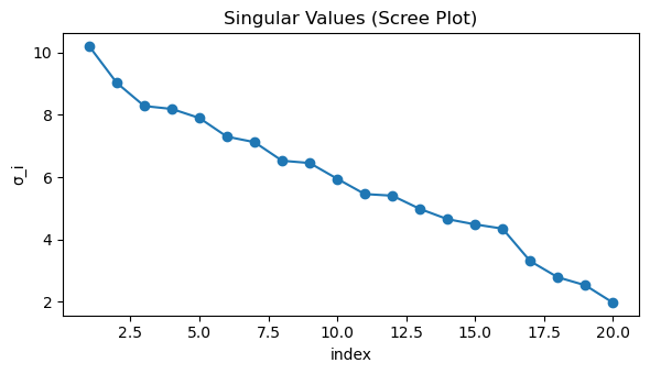
# Scree plot of singular values
plt.figure(figsize=(6, 3.5))
plt.plot(np.arange(1, len(S) + 1), S, marker="o")
plt.title("Singular Values (Scree Plot)")
plt.xlabel("index")
plt.ylabel("σ_i")
plt.tight_layout()
plt.show()
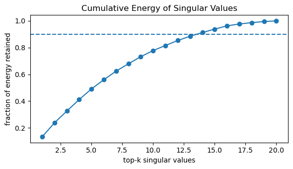
# Cumulative energy plot (how many σ_i capture most variance)
cum_energy = np.cumsum(S**2) / energy_total
plt.figure(figsize=(6, 3.5))
plt.plot(np.arange(1, len(S) + 1), cum_energy, marker="o")
plt.axhline(0.9, linestyle="--") # 90% energy reference
plt.title("Cumulative Energy of Singular Values")
plt.xlabel("top-k singular values")
plt.ylabel("fraction of energy retained")
plt.tight_layout()
plt.show()
Output:
    A shape: (40, 20)
    Top-10 singular values: [10.2052  9.0294  8.2849  8.1918  7.9007  7.3019  7.1258  6.53    6.4572
      5.9514]
    Frobenius ‖A‖_F = 27.9546
    Rank-5 error ‖A - A_k‖_F = 19.9403  (relative 71.33%)
    Energy retained by top 5: 49.12%
    Rank-6 error ‖A - A_k+1‖_F = 18.5552  (should be ≤ rank-5 error)
6. Matrix Calculus — Gradients & Jacobians
Matrix calculus generalizes differentiation to vector and matrix-valued functions. It forms the mathematical backbone of optimization in machine learning and reinforcement learning (RL).
Gradients with Respect to Vectors
For a scalar function $ f(x) = \tfrac{1}{2}|A x - b|_2^2 $, where $A \in \mathbb{R}^{m \times n}$, $x \in \mathbb{R}^n$, and $b \in \mathbb{R}^m$, the gradient is:
\[\nabla_x f = A^\top (A x - b)\]This comes from expanding $f(x) = \tfrac{1}{2}(A x - b)^\top (A x - b)$ and applying the chain rule.
The gradient points in the direction of steepest ascent of $f$, and $-\nabla_x f$ is used for gradient descent.
Gradients with Respect to Matrices
For $ f(W) = \tfrac{1}{2}|W x - y|_2^2 $, with $W \in \mathbb{R}^{m \times n}$, $x \in \mathbb{R}^n$, and $y \in \mathbb{R}^m$:
\[\nabla_W f = (W x - y) x^\top\]This result follows directly from the vector case and the chain rule. Each element of $\nabla_W f$ represents the partial derivative of $f$ with respect to $W_{ij}$.
Jacobian Matrix
For a vector-valued function $ g(x): \mathbb{R}^n \to \mathbb{R}^m $, the Jacobian $ J_g(x) \in \mathbb{R}^{m \times n} $ is defined as:
\[[J_g(x)]_{ij} = \frac{\partial g_i(x)}{\partial x_j}\]It generalizes the derivative to multivariate mappings, encoding how each component of $g$ changes with each component of $x$.
RL Connection
Matrix calculus underpins nearly every gradient-based RL algorithm:
| Concept | Mathematical Role |
|---|---|
| Policy Gradient | Derives updates like \( \nabla_\theta J(\pi_\theta) = \mathbb{E}_\pi[\nabla_\theta \log \pi_\theta(a|s) G_t] \) |
| Backpropagation in Value Networks | Uses Jacobians to propagate derivatives through multiple layers of parameters $W_i$ |
| Actor–Critic Methods | Require computing gradients of expected returns through both policy and value functions |
| Natural Gradients | Use curvature information (Fisher matrix) — an extension of Jacobian-based second-order methods |
In short, matrix calculus is the language of optimization — translating loss functions into actionable gradient updates in reinforcement learning.
Code:
# Gradient wrt vector x
def f_x(x, A, b):
    """Scalar function f(x) = 1/2 * ||A x - b||^2"""
    r = A @ x - b
    return 0.5 * float(r.T @ r)

def grad_x(x, A, b):
    """Analytical gradient ∇x f = Aᵀ(Ax - b)"""
    return A.T @ (A @ x - b)

def numgrad_x(x, A, b, eps=1e-5):
    """Finite-difference approximation of gradient wrt x"""
    g = np.zeros_like(x)
    for i in range(len(x)):
        x1 = x.copy(); x1[i] += eps
        x2 = x.copy(); x2[i] -= eps
        g[i] = (f_x(x1, A, b) - f_x(x2, A, b)) / (2 * eps)
    return g

# Test gradient wrt x
rng = np.random.default_rng(7)
m, n = 30, 4
A = rng.normal(size=(m, n))
x = rng.normal(size=n)
b = rng.normal(size=m)

g_theory = grad_x(x, A, b)
g_num = numgrad_x(x, A, b)

print("∇x_theory =", np.round(g_theory, 6))
print("∇x_num    =", np.round(g_num, 6))
print("‖∇x_theory - ∇x_num‖₂ =", np.linalg.norm(g_theory - g_num))

# Gradient wrt matrix W
def f_W(W, x, y):
    """Scalar function f(W) = 1/2 * ||W x - y||^2"""
    r = W @ x - y
    return 0.5 * float(r.T @ r)

def grad_W(W, x, y):
    """Analytical gradient ∇W f = (W x - y) xᵀ"""
    r = W @ x - y
    return np.outer(r, x)

def numgrad_W(W, x, y, eps=1e-5):
    """Finite-difference approximation of gradient wrt each element W[i,j]"""
    G = np.zeros_like(W)
    for i in range(W.shape[0]):
        for j in range(W.shape[1]):
            W1 = W.copy(); W1[i, j] += eps
            W2 = W.copy(); W2[i, j] -= eps
            G[i, j] = (f_W(W1, x, y) - f_W(W2, x, y)) / (2 * eps)
    return G

# Test gradient wrt W
rng = np.random.default_rng(8)
m, n = 5, 3
W = rng.normal(size=(m, n))
x = rng.normal(size=n)
y = rng.normal(size=m)

G_theory = grad_W(W, x, y)
G_num = numgrad_W(W, x, y)

print("\n∇W_theory =\n", np.round(G_theory, 6))
print("∇W_num    =\n", np.round(G_num, 6))
print("‖∇W_theory - ∇W_num‖_F =", np.linalg.norm(G_theory - G_num))
Output:
∇x_theory = [-18.687021  -1.964063 -15.837229 -63.186924]
∇x_num    = [-18.687021  -1.964063 -15.837229 -63.186924]
‖∇x_theory - ∇x_num‖₂ = 2.7846929469737626e-09

∇W_theory =
 [[-1.298238  0.090769 -3.062965]
 [-0.052729  0.003687 -0.124406]
 [ 0.239965 -0.016778  0.566154]
 [ 0.29452  -0.020592  0.694868]
 [ 0.70727  -0.04945   1.668681]]
∇W_num    =
 [[-1.298238  0.090769 -3.062965]
 [-0.052729  0.003687 -0.124406]
 [ 0.239965 -0.016778  0.566154]
 [ 0.29452  -0.020592  0.694868]
 [ 0.70727  -0.04945   1.668681]]
‖∇W_theory - ∇W_num‖_F = 3.381426609910155e-11
7. Chain Rule & Backpropagation
The chain rule is the backbone of backpropagation — the mechanism that allows deep neural networks to learn. It lets us compute gradients of composite functions efficiently by applying local derivatives layer by layer.
Theoretical Setup
Consider a two-layer (nonlinear) mapping:
\[f(x) = W_2 \, \sigma(W_1 x),\]where:
- $x \in \mathbb{R}^{n}$ is the input,
- $W_1 \in \mathbb{R}^{h \times n}$ and $W_2 \in \mathbb{R}^{m \times h}$ are weight matrices,
- $\sigma(\cdot)$ is an elementwise nonlinearity (e.g., $\tanh$).
We define a simple loss function:
\[L = \tfrac{1}{2} \| f(x) - y \|^2,\]where $y \in \mathbb{R}^m$ is the target output.
Analytical Gradients
Let:
\[h = \tanh(W_1 x), \quad f(x) = W_2 h.\]Then, the gradients follow from the chain rule:
\[\nabla_{W_2} L = (f(x) - y) \, h^\top,\] \[\nabla_{W_1} L = \Big( W_2^\top (f(x) - y) \odot (1 - h^2) \Big) x^\top.\]Here:
- $ \odot $ denotes elementwise multiplication,
- $ (1 - h^2) $ is the derivative of $\tanh(z)$,
- The first term backpropagates the error through the linear and nonlinear layers.
These equations are exactly what automatic differentiation computes under the hood in frameworks like PyTorch or TensorFlow.
RL Connection
Backpropagation is central to modern RL — particularly policy-gradient and actor–critic methods — because it allows agents to learn from differentiable signals.
| RL Concept | Backpropagation Role |
|---|---|
| Policy Networks | Gradients of $ \log \pi_\theta(a \mid s) $ are computed via backprop. |
| Value Function Approximation | Gradients of mean-squared error loss $ (V_\theta(s) - G_t)^2 $ use the same chain rule. |
| Actor–Critic Updates | The critic’s backpropagated signal informs the actor’s gradient direction. |
| End-to-End Differentiable Agents | From state embeddings to reward models — all components train using backpropagation. |
Code:
# Forward / Loss / Analytic Gradients
def forward(W1, W2, x):
    h = np.tanh(W1 @ x) # hidden
    yhat = W2 @ h # output (linear)
    return yhat, h

def loss(W1, W2, x, y):
    yhat, _ = forward(W1, W2, x)
    r = yhat - y
    return 0.5 * float(r @ r) # 1/2 ||yhat - y||^2

def grad_Ws(W1, W2, x, y):
    yhat, h = forward(W1, W2, x)
    r  = yhat - y # (m,)
    dW2 = np.outer(r, h) # (m,h)
    dh  = W2.T @ r # (h,)
    dW1 = np.outer(dh * (1.0 - h**2), x) # (h,n)  since d/dz tanh(z)=1-tanh^2(z)
    return dW1, dW2

# Numerical Gradient (central difference)
def numgrad_mat(fun, W, eps=1e-5):
    G = np.zeros_like(W)
    for idx in np.ndindex(*W.shape):
        W1 = W.copy(); W1[idx] += eps
        W2 = W.copy(); W2[idx] -= eps
        G[idx] = (fun(W1) - fun(W2)) / (2.0 * eps)
    return G

# Helper: report absolute and relative errors
def grad_report(name, G_th, G_num, atol=1e-6, rtol=1e-6):
    diff = G_th - G_num
    abs_err = np.linalg.norm(diff) # Frobenius/2-norm
    rel_den = max(1.0, np.linalg.norm(G_th), np.linalg.norm(G_num))
    rel_err = abs_err / rel_den
    max_abs = float(np.max(np.abs(diff)))
    print(f"{name}: ‖th - num‖ = {abs_err:.3e} | rel = {rel_err:.3e} | max|diff| = {max_abs:.3e}")

# Testing with a fixed seed
rng = np.random.default_rng(9)
h, n, m = 6, 4, 3 # hidden, in_dim, out_dim
W1 = 0.5 * rng.normal(size=(h, n))
W2 = 0.5 * rng.normal(size=(m, h))
x  = rng.normal(size=n)
y  = rng.normal(size=m)

# Analytic grads
dW1, dW2 = grad_Ws(W1, W2, x, y)

# Numerical grads (central differences)
fW1 = lambda W: loss(W, W2, x, y)
fW2 = lambda W: loss(W1, W, x, y)
dW1_num = numgrad_mat(fW1, W1, eps=1e-5)
dW2_num = numgrad_mat(fW2, W2, eps=1e-5)

# Reports
grad_report("∇W1", dW1, dW1_num)
grad_report("∇W2", dW2, dW2_num)
Output:
∇W1: ‖th - num‖ = 1.032e-10 | rel = 4.147e-11 | max|diff| = 3.390e-11
∇W2: ‖th - num‖ = 5.212e-11 | rel = 1.369e-11 | max|diff| = 2.585e-11
Key Takeaways
- Vectors, Matrices, and Norms — build the language for representing data and transformations.
- Linear Systems & Least Squares — form the basis of value-function approximation and regression.
- Eigenvalues & SVD — reveal structure, stability, and low-rank approximations in RL models.
- Matrix Calculus & Backpropagation — provide the mathematical backbone for gradient-based learning.
- Chain Rule — powers end-to-end differentiable optimization in modern RL and deep learning.
Linear algebra and matrix calculus are the foundation of neural function approximation, gradient-based policy updates, and value estimation in reinforcement learning.
Next: 02_gradient_descent_optimize.ipynb → implement optimization from first principles: gradients, learning rate, convergence, and visualization of loss surfaces.