Gradient Descent & Optimization

A practical, visual guide to first-order optimization — from vanilla GD to Adam — with RL connections.

What you’ll learn

Gradient Descent, step size, convergence on quadratics
Momentum & Nesterov acceleration — intuition and practice
Adaptive methods: AdaGrad, RMSProp, Adam
Schedules, gradient clipping, plateaus / exploding gradients
Reinforcement Learning connections — policy gradient stability, critic regression, entropy/weight decay

How to use: Skim the theory blocks, then run the code cells — each section includes small, focused demos.

1. Vanilla Gradient Descent (GD)

Gradient Descent (GD) is the core optimization algorithm underlying almost every modern machine learning and reinforcement learning (RL) method. It iteratively updates parameters in the opposite direction of the gradient to minimize a loss function.

Definition

Given a differentiable function $ f:\mathbb{R}^n \rightarrow \mathbb{R} $, the gradient descent update rule is:

\[x_{k+1} = x_k - \eta \, \nabla f(x_k),\]

where $ \eta > 0 $ is the learning rate (step size).

If $ \eta $ is too small, convergence is slow.
If $ \eta $ is too large, the algorithm may overshoot and diverge.

Convergence on Quadratics

For quadratic functions of the form

\[f(x) = \tfrac{1}{2}x^\top Q x + b^\top x + c, \quad Q \succ 0,\]

gradient descent converges linearly if

\[0 < \eta < \frac{2}{L}, \quad \text{where } L = \lambda_{\max}(Q).\]

The optimal constant step size for convergence is approximately:

\[\eta^* = \frac{2}{\lambda_{\min}(Q) + \lambda_{\max}(Q)}.\]

Here:

$ \lambda_{\max}(Q) $: maximum eigenvalue (steepest curvature)
$ \lambda_{\min}(Q) $: minimum eigenvalue (flattest curvature)
$ \kappa = \frac{\lambda_{\max}}{\lambda_{\min}} $: condition number, which determines how “stretched” the loss surface is.

Intuition:
A large condition number ($\kappa \gg 1$) causes zig-zagging updates along steep directions — a common reason for slow convergence and oscillations.

Visualization Intuition

On an elliptical loss surface (like $x^\top Q x$):

Each step moves downhill along the negative gradient.
The learning rate $\eta$ controls how far we move each time.
Good step sizes lead to smooth spiraling toward the minimum.

RL Connection

In Reinforcement Learning, gradient descent forms the foundation of:

Concept	Description	Gradient Interpretation
Policy Optimization	Adjusting parameters to maximize expected return.	$ \theta_{k+1} = \theta_k + \eta \, \nabla_\theta J(\pi_\theta) $
Value Function Approximation	Fitting value networks via TD-error or MSE.	$ w_{k+1} = w_k - \eta \, \nabla_w \tfrac{1}{2}(V_w - \hat V)^2 $
Actor–Critic Updates	Policy and value updates alternate using gradient signals.	Separate learning rates stabilize learning
Stability Considerations	Too large a step can cause divergence (e.g., Q-learning instability).	Proper scheduling of $\eta$ is crucial

Code:

# Gradient Descent on a 2D Quadratic: stability vs. step size (fixed visuals)
import numpy as np
import matplotlib.pyplot as plt

Q = np.array([[5.0, 0.0],
              [0.0, 1.0]])

def f(x):   return 0.5 * x @ Q @ x
def grad(x): return Q @ x

eigvals = np.linalg.eigvalsh(Q)
mu, L = eigvals[0], eigvals[-1]
eta_star = 2.0 / (mu + L)
eta_max  = 2.0 / L

print(f"λ_min={mu:.3f}, λ_max={L:.3f}, κ={L/mu:.2f}")
print(f"η* (optimal fixed step) ≈ {eta_star:.3f}")
print(f"Stability requires 0 < η < {eta_max:.3f}")

def run_gd(x0, lr, steps=200):
    x = x0.copy()
    xs = [x.copy()]
    vals = [f(x)]
    for _ in range(steps):
        x = x - lr * grad(x)
        xs.append(x.copy())
        vals.append(f(x))
    return np.array(xs), np.array(vals)

x0 = np.array([3.0, -3.0])

# Choose LR: conservative, near-optimal, slightly-unstable (just above 2/L = 0.4)
lrs    = [0.10, eta_star, 0.41]
labels = [f"η={lrs[0]:.2f} (small)",
          f"η≈η*={lrs[1]:.3f} (near-optimal)",
          f"η={lrs[2]:.2f} (> 2/λ_max ⇒ unstable)"]

runs = [run_gd(x0, lr) for lr in lrs]

# Contours + trajectories (clip view, trim diverging path)
view = 3.5
grid = np.linspace(-view, view, 220)
X, Y = np.meshgrid(grid, grid)
Z = 0.5*(Q[0,0]*X**2 + 2*Q[0,1]*X*Y + Q[1,1]*Y**2)

plt.figure(figsize=(6.4, 5.2))
cs = plt.contour(X, Y, Z, levels=20)
plt.clabel(cs, inline=True, fontsize=8)

colors = ["tab:blue", "tab:orange", "tab:green"]
for (path, vals), lab, col in zip(runs, labels, colors):
    # If the run diverges, plot only the first K in-bounds steps to avoid autoscale blow-up
    in_bounds = np.all(np.abs(path) <= view, axis=1)
    if in_bounds.sum() == len(path):
        # stable: plot all
        plt.plot(path[:,0], path[:,1], marker="o", markersize=2, label=lab, color=col)
    else:
        # unstable: plot only first chunk inside the view window
        k = np.argmax(~in_bounds) # first out-of-bounds index
        k = max(k, 2) # at least two points to draw a segment
        plt.plot(path[:k,0], path[:k,1], marker="o", markersize=2, label=lab, color=col, alpha=0.9)
        # indicate it diverged
        last = path[k-1]
        plt.scatter(last[0], last[1], s=40, color=col, marker="x", zorder=3)
        plt.text(last[0], last[1], " diverged →", fontsize=9, color=col, va="center")

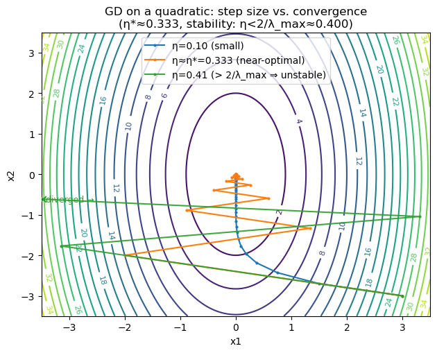
plt.title(f"GD on a quadratic: step size vs. convergence\n(η*≈{eta_star:.3f}, stability: η<2/λ_max≈{eta_max:.3f})")
plt.xlabel("x1"); plt.ylabel("x2")
plt.xlim(-view, view); plt.ylim(-view, view)
plt.legend()
plt.tight_layout()
plt.show()

Output:

λ_min=1.000, λ_max=5.000, κ=5.00
η* (optimal fixed step) ≈ 0.333
Stability requires 0 < η < 0.400

png

2. Momentum & Nesterov Acceleration

Gradient Descent can oscillate on valleys or ill-conditioned surfaces. Momentum adds an inertial term that helps the optimizer move faster along consistent directions and dampen oscillations across steep walls.

Momentum

We maintain a velocity vector $v_k$ that accumulates past gradients:

\[v_{k+1} = \beta v_k + \nabla f(x_k), \qquad x_{k+1} = x_k - \eta v_{k+1},\]

where

$ \beta \in [0,1) $ is the momentum coefficient (typically 0.9),
$ \eta $ is the learning rate.

Intuition:

The update combines the current gradient with a fraction of the previous direction.
Like pushing a ball down a hill — once it gains speed, small bumps don’t stop it.

Nesterov Accelerated Gradient (NAG)

Nesterov’s idea is to look ahead before computing the gradient, giving smoother convergence:

\[v_{k+1} = \beta v_k + \nabla f(x_k - \eta \beta v_k), \qquad x_{k+1} = x_k - \eta v_{k+1}.\]

This “anticipatory” step makes NAG more stable and responsive — the optimizer slows down automatically near minima.

Geometric Intuition

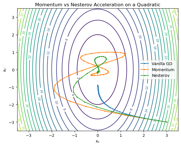
Momentum smooths oscillations in narrow ravines.
NAG further improves by predicting where the next step will be.
Both reduce the zig-zag effect in poorly conditioned loss landscapes.

RL Connection

RL Concept	Optimization Analogy
Policy updates	Momentum helps stabilize noisy gradients from sampled trajectories.
Value network training	NAG accelerates convergence when value loss surfaces are elongated.
Actor–critic learning	Critic updates can benefit from velocity terms to reduce variance in gradient flow.
Adaptive methods (e.g., Adam)	Combine momentum with per-parameter scaling for robust RL training.

Momentum-based optimizers are crucial in RL because policy gradients are noisy and high-variance — accumulating direction information leads to smoother and faster learning.

Code:

def run_optimizer(x0, lr, beta, steps=50, mode="momentum"):
    x = x0.copy()
    v = np.zeros_like(x)
    xs, vals = [x.copy()], [f(x)]
    for _ in range(steps):
        if mode == "momentum":
            v = beta * v + grad(x)
            x = x - lr * v
        elif mode == "nesterov":
            v = beta * v + grad(x - lr * beta * v)
            x = x - lr * v
        else:
            x = x - lr * grad(x)
        xs.append(x.copy())
        vals.append(f(x))
    return np.array(xs), np.array(vals)

x0 = np.array([3.0, -3.0])
lr = 0.024
beta = 0.9

runs = {
    "Vanilla GD": run_optimizer(x0, lr, beta, mode="gd"),
    "Momentum":   run_optimizer(x0, lr, beta, mode="momentum"),
    "Nesterov":   run_optimizer(x0, lr, beta, mode="nesterov")
}

# Contour plot with trajectories
grid = np.linspace(-3.5, 3.5, 200)
X, Y = np.meshgrid(grid, grid)
Z = 0.5 * (Q[0,0]*X**2 + 2*Q[0,1]*X*Y + Q[1,1]*Y**2)

plt.figure(figsize=(6.4, 5.2))
cs = plt.contour(X, Y, Z, levels=20)
plt.clabel(cs, inline=True, fontsize=8)

colors = ["tab:blue", "tab:orange", "tab:green"]
for (name, (path, vals)), c in zip(runs.items(), colors):
    plt.plot(path[:,0], path[:,1], marker="o", markersize=2, label=name, color=c)
plt.title("Momentum vs Nesterov Acceleration on a Quadratic")
plt.xlabel("x₁"); plt.ylabel("x₂")
plt.legend()
plt.tight_layout()
plt.show()

png

3. Adaptive Methods — AdaGrad, RMSProp, Adam

Classical Gradient Descent uses a single global learning rate $ \eta $ for all parameters. However, different parameters may experience gradients of vastly different magnitudes. Adaptive methods address this by scaling updates using historical gradient information.

AdaGrad

AdaGrad (Duchi et. al, 2011) accumulates the squared gradients for each parameter:

\[g_t = \nabla_\theta f_t, \qquad G_t = G_{t-1} + g_t^2, \qquad \theta_{t+1} = \theta_t - \frac{\eta}{\sqrt{G_t + \epsilon}} g_t.\]

Coordinates with large gradients get smaller effective learning rates.
Works well for sparse features (e.g., text, embeddings).
Drawback: the accumulated $G_t$ keeps growing, causing vanishing steps.

RMSProp

RMSProp (Hinton, 2012) fixes AdaGrad’s decay issue by using an exponential moving average:

\[v_t = \beta v_{t-1} + (1-\beta) g_t^2, \qquad \theta_{t+1} = \theta_t - \frac{\eta}{\sqrt{v_t + \epsilon}} g_t.\]

Smooths the gradient magnitude estimate.
Prevents aggressive decay in learning rate.
Common in non-stationary settings like RL.

Adam

Adam (Kingma et. al, 2014) combines Momentum and RMSProp — tracking both first and second moments:

\[\begin{aligned} m_t &= \beta_1 m_{t-1} + (1-\beta_1) g_t, \\ v_t &= \beta_2 v_{t-1} + (1-\beta_2) g_t^2, \\ \hat{m}_t &= \frac{m_t}{1-\beta_1^t}, \qquad \hat{v}_t = \frac{v_t}{1-\beta_2^t}, \\ \theta_{t+1} &= \theta_t - \eta \frac{\hat{m}_t}{\sqrt{\hat{v}_t} + \epsilon}. \end{aligned}\]

Momentum improves stability.
RMS scaling ensures robust adaptation.
Bias correction keeps early updates consistent.

RL Connection

RL Concept	Optimizer Analogy
Policy Gradient Updates	Adam stabilizes noisy, high-variance policy gradients across episodes.
Value Function Fitting	RMSProp smooths non-stationary TD errors, aiding stable critic updates.
Actor–Critic Methods	Separate step-size adaptation for actor and critic encourages balanced learning.
Exploration in Noisy Environments	Adaptive step scaling helps avoid premature convergence to suboptimal policies.

Code:

# Optimizer steps
def adagrad_step(x, g, G, lr=0.30, eps=1e-8):
    G = G + g*g
    x = x - lr * g / (np.sqrt(G) + eps)
    return x, G

def rmsprop_step(x, g, v, lr=0.20, beta=0.9, eps=1e-8):
    v = beta*v + (1-beta)*(g*g)
    x = x - lr * g / (np.sqrt(v) + eps)
    return x, v

def adam_step(x, g, m, v, t, lr=0.15, b1=0.9, b2=0.999, eps=1e-8):
    m = b1*m + (1-b1)*g
    v = b2*v + (1-b2)*(g*g)
    mhat = m / (1 - b1**t)
    vhat = v / (1 - b2**t)
    x = x - lr * mhat / (np.sqrt(vhat) + eps)
    return x, m, v

# Runners
def run_adagrad(x0, steps=80, lr=0.30, noise_std=0.10, clip_norm=None, seed=0):
    x = x0.astype(float).copy()
    G = np.zeros_like(x)
    rng = np.random.default_rng(seed)
    xs = [x.copy()]; losses = [f(x)]
    for _ in range(1, steps+1):
        g = grad(x) + noise_std * rng.normal(size=x.shape)
        if clip_norm:
            n = np.linalg.norm(g)
            if n > clip_norm: g *= (clip_norm/n)
        x, G = adagrad_step(x, g, G, lr=lr)
        xs.append(x.copy()); losses.append(f(x))
    return np.array(xs), np.array(losses)

def run_rmsprop(x0, steps=80, lr=0.20, beta=0.9, noise_std=0.10, clip_norm=None, seed=1):
    x = x0.astype(float).copy()
    v = np.zeros_like(x)
    rng = np.random.default_rng(seed)
    xs = [x.copy()]; losses = [f(x)]
    for _ in range(1, steps+1):
        g = grad(x) + noise_std * rng.normal(size=x.shape)
        if clip_norm:
            n = np.linalg.norm(g)
            if n > clip_norm: g *= (clip_norm/n)
        x, v = rmsprop_step(x, g, v, lr=lr, beta=beta)
        xs.append(x.copy()); losses.append(f(x))
    return np.array(xs), np.array(losses)

def run_adam(x0, steps=80, lr=0.15, b1=0.9, b2=0.999, noise_std=0.10, clip_norm=None, seed=2):
    x = x0.astype(float).copy()
    m = np.zeros_like(x); v = np.zeros_like(x)
    rng = np.random.default_rng(seed)
    xs = [x.copy()]; losses = [f(x)]
    for t in range(1, steps+1):
        g = grad(x) + noise_std * rng.normal(size=x.shape)
        if clip_norm:
            n = np.linalg.norm(g)
            if n > clip_norm: g *= (clip_norm/n)
        x, m, v = adam_step(x, g, m, v, t, lr=lr, b1=b1, b2=b2)
        xs.append(x.copy()); losses.append(f(x))
    return np.array(xs), np.array(losses)

# Run all three on the same problem
x0 = np.array([3.0, -3.0])
paths = {}
losses = {}

paths["AdaGrad"], losses["AdaGrad"]   = run_adagrad(x0, lr=0.25, noise_std=0.10, clip_norm=5.0)
paths["RMSProp"], losses["RMSProp"]   = run_rmsprop(x0, lr=0.075, beta=0.9, noise_std=0.10, clip_norm=5.0)
paths["Adam"],    losses["Adam"]      = run_adam(x0, lr=0.05, b1=0.9, b2=0.999, noise_std=0.10, clip_norm=5.0)

print("AdaGrad LR: 0.25, RMSProp LR: 0.075, Adam LR: 0.05")

# Contours + trajectories
view = 3.5
grid = np.linspace(-view, view, 220)
X, Y = np.meshgrid(grid, grid)
Z = 0.5*(Q[0,0]*X**2 + 2*Q[0,1]*X*Y + Q[1,1]*Y**2)

plt.figure(figsize=(6.6, 5.2))
cs = plt.contour(X, Y, Z, levels=20)
plt.clabel(cs, inline=True, fontsize=8)
colors = {"AdaGrad":"tab:blue", "RMSProp":"tab:orange", "Adam":"tab:green"}
for name in ["AdaGrad","RMSProp","Adam"]:
    p = paths[name]
    plt.plot(p[:,0], p[:,1], marker="o", markersize=2, label=name, color=colors[name])
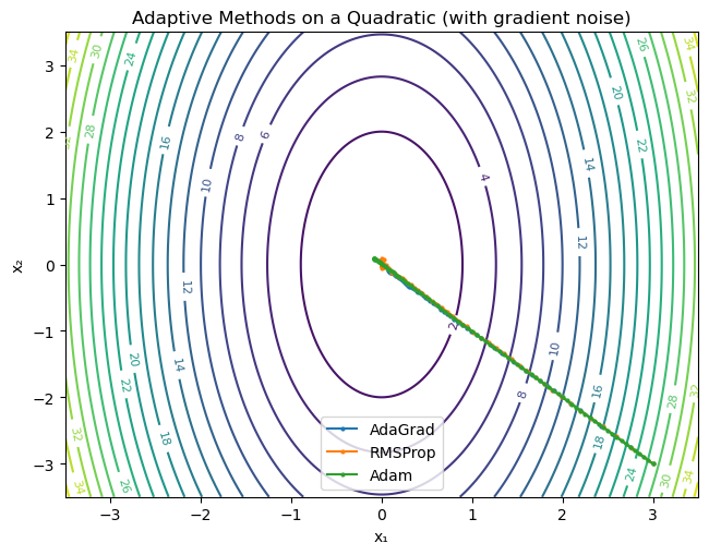
plt.title("Adaptive Methods on a Quadratic (with gradient noise)")
plt.xlabel("x₁"); plt.ylabel("x₂"); plt.xlim(-view, view); plt.ylim(-view, view)
plt.legend(); plt.tight_layout(); plt.show()

Output:

AdaGrad LR: 0.25, RMSProp LR: 0.075, Adam LR: 0.05

png

4. Schedules, Gradient Clipping, and Plateaus

Learning Rate (LR) Schedules

A learning rate schedule adjusts the step size $\eta_k$ during training to balance exploration (large steps early) and convergence (smaller steps later).
Common schedules:

\[\eta_k = \begin{cases} \eta_0 \cdot \gamma^{\lfloor k / s \rfloor}, & \text{(step decay)} \\ \eta_0 \cdot \frac{1}{\sqrt{k}}, & \text{(inverse-square-root decay)} \\ \eta_0 \cdot \frac{1}{2}\big(1 + \cos(\pi k / K)\big), & \text{(cosine decay)} \end{cases}\]

Large learning rates help escape flat regions or plateaus early on.
Gradual decay prevents oscillations near optima.
Warm restarts (e.g., cosine annealing) cyclically increase $\eta_k$ to promote exploration again.

Gradient Clipping

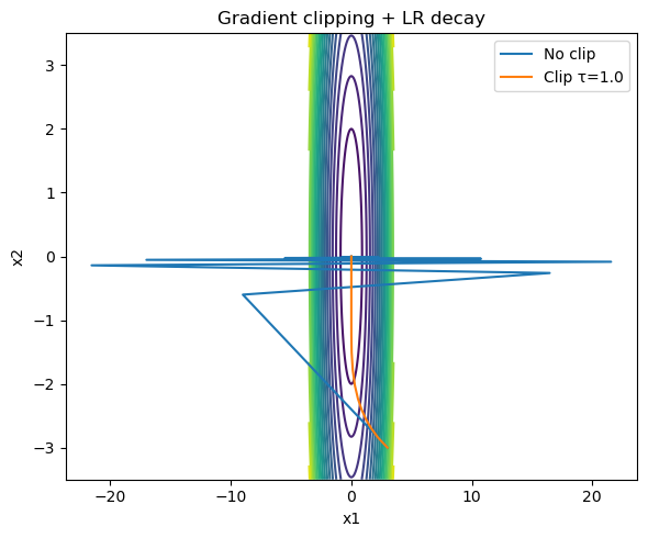
To prevent instability when gradients explode, we clip the gradient norm:

\[g \leftarrow g \cdot \frac{\tau}{\|g\|_2}, \quad \text{if } \|g\|_2 > \tau.\]

Stabilizes training in deep or recurrent networks.
Prevents large parameter updates that could derail optimization.

Plateaus and Flat Regions

During training, gradients may approach zero even far from optimality (common in sigmoid/tanh activations or deep credit assignment). Adaptive LR and momentum methods help “push through” these flat regions by maintaining accumulated update momentum or increasing effective step sizes.

RL Connection

RL Concept	Optimization Analogy
Policy Gradient Training	LR schedules prevent premature convergence to suboptimal deterministic policies.
Value Function Updates	Clipping gradients stabilizes critic learning when TD errors explode.
Actor–Critic Stability	Small LR for critic, larger for actor — prevents feedback loops.
Exploration Plateaus	LR restarts or adaptive scaling can reintroduce exploration after stagnation.

In practice, Adam with gradient clipping and cosine decay LR schedules are standard for modern deep RL algorithms (e.g., PPO, SAC, DDPG).

Code:

def run_gd_clip(x0, lr, steps=60, clip=None):
    x = x0.copy(); xs=[x.copy()]
    for k in range(1, steps+1):
        g = grad(x)
        if clip is not None:
            n = np.linalg.norm(g)
            if n > clip: g = g * (clip / n)
        eta = lr / np.sqrt(k)   # simple decay
        x = x - eta * g
        xs.append(x.copy())
    return np.array(xs)

clip_path = run_gd_clip(np.array([3.0,-3.0]), lr=0.8, steps=80, clip=1.0)
noclip_path = run_gd_clip(np.array([3.0,-3.0]), lr=0.8, steps=80, clip=None)

plt.figure(figsize=(6,5))
cs = plt.contour(X, Y, Z, levels=20)
plt.plot(noclip_path[:,0], noclip_path[:,1], label="No clip")
plt.plot(clip_path[:,0], clip_path[:,1], label="Clip τ=1.0")
plt.legend(); plt.title("Gradient clipping + LR decay")
plt.xlabel("x1"); plt.ylabel("x2"); plt.tight_layout(); plt.show()

png

5. RL Tie-Ins — Policy Gradient & Critic Regression

Optimization is at the core of reinforcement learning — every policy or value function update ultimately involves minimizing or maximizing an objective via gradient-based methods.

Policy Gradient — Maximizing Expected Return

The policy gradient theorem provides a principled way to adjust parameters $\theta$ of a stochastic policy $\pi_\theta(a \mid s)$ to maximize expected cumulative reward:

\[J(\theta) = \mathbb{E}_{\pi_\theta}\Big[\sum_{t=0}^{\infty} \gamma^t R_t\Big].\]

The gradient is:

\[\nabla_\theta J(\theta) = \mathbb{E}_{\pi_\theta}\!\big[\,\nabla_\theta \log \pi_\theta(a \mid s) \, G_t\,\big],\]

where $G_t$ is the discounted return.
In practice, we estimate this via Monte Carlo samples:

\[\theta \leftarrow \theta + \eta \, \nabla_\theta \log \pi_\theta(a_t \mid s_t) \, G_t.\]

Connection to optimization:

It’s stochastic gradient ascent on $J(\theta)$.
Techniques like momentum, Adam, and gradient clipping directly transfer here.
LR schedules help stabilize policy updates and reduce variance.

Critic Regression — Minimizing Value Error

The critic (value function approximator) is trained to minimize the mean-squared error between predicted and empirical returns:

\[L(\phi) = \tfrac{1}{2}\, \mathbb{E}\big[(V_\phi(s_t) - G_t)^2\big].\]

The gradient is:

\[\nabla_\phi L = (V_\phi(s_t) - G_t) \, \nabla_\phi V_\phi(s_t),\]

which is optimized using standard gradient descent or Adam.

Connection to optimization:

Equivalent to supervised regression.
Often uses smaller learning rates than the policy to ensure stable updates.
Adaptive methods (Adam) handle noisy value targets well.

Summary Table

RL Component	Objective	Optimization Type	Update Rule
Actor (Policy)	Maximize expected return $J(\theta)$	Gradient ascent	$\theta \leftarrow \theta + \eta \nabla_\theta \log \pi_\theta(a \mid s) G_t$
Critic (Value Function)	Minimize MSE $L(\phi)$	Gradient descent	$\phi \leftarrow \phi - \eta (V_\phi - G_t)\nabla_\phi V_\phi$

Key Takeaways

Step size controls stability; conditioning dictates GD speed on quadratics.
Momentum/Nesterov reduce oscillations and speed up progress on ill-conditioned problems.
Adaptive optimizers (Adam/RMSProp/AdaGrad) tune per-parameter steps and handle noise.
Schedules & clipping mitigate exploding/vanishing gradients and plateaus.
In RL, these tools stabilize policy gradients and critic training.

Next: 03_scikit-learn_basics.ipynb → learn about regression, classification, and hyperparameter search using scikit-learn library.