Dynamic Programming: Policy Iteration
From arbitrary behavior to optimal policies via alternating evaluation and improvement.
What you’ll learn
- How policy evaluation and policy improvement combine into policy iteration.
- How to implement policy iteration on the classic 4×4 Gridworld.
- How to visualize value functions and policies (arrows) on a grid.
- Why policy iteration converges to the optimal policy in finite MDPs.
This notebook assumes you’ve seen:
11_markov_decision_processes.ipynb,12_bellman_equations.ipynb, and13_dp_policy_evaluation.ipynb.
1. Theory — Policy Evaluation + Policy Improvement
We work with a finite discounted MDP with states $ \mathcal{S} $, actions $ \mathcal{A} $, transition dynamics $ p(s’, r \mid s, a) $, and discount $ \gamma \in [0,1) $.
A policy $ \pi(a \mid s) $ defines a distribution over actions for each state.
1.1 Policy Evaluation (Reminder)
Given a policy $ \pi $, the state-value function $ v_\pi $ satisfies the Bellman expectation equation:
\[v_\pi(s) = \mathbb{E}_\pi \big[ R_{t+1} + \gamma v_\pi(S_{t+1}) \mid S_t = s \big] = \sum_a \pi(a\mid s) \sum_{s',r} p(s',r\mid s,a)\,\big[r + \gamma v_\pi(s')\big].\]In matrix form (for Markov reward processes / fixed policy):
\[v_\pi = r^\pi + \gamma P^\pi v_\pi \quad \Longrightarrow \quad v_\pi = (I - \gamma P^\pi)^{-1} r^\pi.\]We typically solve this iteratively using dynamic programming (DP):
\[v_{k+1}(s) \leftarrow \sum_a \pi(a\mid s) \sum_{s'} P(s' \mid s, a) \big[R(s,a,s') + \gamma v_k(s')\big].\]1.2 Policy Improvement
If we have $ v_\pi $, we can define the state–action value:
\[q_\pi(s,a) = \sum_{s',r} p(s',r\mid s,a)\,\big[r + \gamma v_\pi(s')\big].\]A greedy policy w.r.t. $ v_\pi $ is:
\[\pi'(s) = \arg\max_a q_\pi(s,a).\]The Policy Improvement Theorem says:
If for all $s$, $ q_\pi(s, \pi’(s)) \ge v_\pi(s) $, then $ v_{\pi’}(s) \ge v_\pi(s) $ for all $s$, and strictly better in some state if inequality is strict somewhere.
So greedy improvement never makes the policy worse.
1.3 Policy Iteration Algorithm
Policy iteration alternates:
- Policy Evaluation: Find $ v_\pi $ for current policy $ \pi $.
- Policy Improvement: Greedify w.r.t. $ v_\pi $ to obtain $ \pi’ $.
Pseudocode (deterministic policies):
Initialize π(s) arbitrarily for all s
loop:
    # Policy Evaluation
    compute v_π (e.g., iterative DP until convergence)

    # Policy Improvement
    policy_stable = True
    for each state s:
        old_action = π(s)
        π(s) = argmax_a q_π(s,a)
        if π(s) != old_action:
            policy_stable = False

    if policy_stable:
        return π, v_π   # π is optimal
For finite discounted MDPs, this converges to an optimal policy $ \pi^* $ in a finite number of iterations.
2. Environment Setup — 4×4 Gridworld (Sutton-style)
Code:
import numpy as np
import matplotlib.pyplot as plt

np.set_printoptions(precision=3, suppress=True)

# We use a 4x4 Gridworld:
# - States: 0..15 laid out row-wise
# - Terminals: 0 (top-left) and 15 (bottom-right)
# - Actions: 0=up, 1=right, 2=down, 3=left
# - Reward: -1 per step until reaching a terminal
# - Discount: gamma

GRID_H = 4
GRID_W = 4
N_STATES = GRID_H * GRID_W
ACTIONS = np.array([0, 1, 2, 3])  # up, right, down, left
N_ACTIONS = len(ACTIONS)

TERMINAL_STATES = {0, N_STATES - 1}


def state_to_coord(s):
    return divmod(s, GRID_W)  # (row, col)


def coord_to_state(i, j):
    return i * GRID_W + j


def step_grid(s, a):
    """Deterministic transition for the grid. Returns (s', reward, done)."""
    if s in TERMINAL_STATES:
        return s, 0.0, True

    i, j = state_to_coord(s)
    if a == 0:      # up
        i = max(i - 1, 0)
    elif a == 1:    # right
        j = min(j + 1, GRID_W - 1)
    elif a == 2:    # down
        i = min(i + 1, GRID_H - 1)
    elif a == 3:    # left
        j = max(j - 1, 0)

    s_next = coord_to_state(i, j)
    reward = -1.0
    done = s_next in TERMINAL_STATES
    return s_next, reward, done


def build_tabular_mdp(gamma=1.0):
    """
    Build P and R for the gridworld MDP.

    P[s, a, s'] = probability of transitioning from s to s' under action a.
    R[s, a]     = expected immediate reward for (s,a).
    """
    P = np.zeros((N_STATES, N_ACTIONS, N_STATES), dtype=float)
    R = np.zeros((N_STATES, N_ACTIONS), dtype=float)

    for s in range(N_STATES):
        for ai, a in enumerate(ACTIONS):
            s_next, r, done = step_grid(s, a)
            P[s, ai, s_next] = 1.0
            R[s, ai] = r

    return P, R, gamma


P, R, gamma = build_tabular_mdp(gamma=1.0)

print("P shape:", P.shape)
print("R shape:", R.shape)
print("Terminal states:", TERMINAL_STATES)
Output:
P shape: (16, 4, 16)
R shape: (16, 4)
Terminal states: {0, 15}
3. Policy Evaluation Helper (Deterministic Policies)
We’ll reuse iterative policy evaluation, but specialized for deterministic policies:
- Policy is represented as an integer array
policy[s] ∈ {0,1,2,3}. - For each non-terminal state $s$, we apply its chosen action, compute its 1-step return, and iterate until convergence:
We stop when the max change across states drops below a threshold theta.
Code:
def evaluate_policy(P, R, gamma, policy, theta=1e-4, max_iters=10_000, verbose=False):
    """
    Iterative policy evaluation for a deterministic policy on the gridworld.

    Args:
        P: (S, A, S) transition probabilities
        R: (S, A) rewards
        gamma: discount factor
        policy: (S,) int array of actions
        theta: convergence tolerance
        max_iters: safety cap
    Returns:
        v: (S,) value function for this policy
        num_iters: number of sweeps performed
    """
    S, A, _ = P.shape
    v = np.zeros(S, dtype=float)

    for it in range(max_iters):
        delta = 0.0
        v_new = v.copy()

        for s in range(S):
            if s in TERMINAL_STATES:
                continue

            a = policy[s]
            # One-step expectation: v(s) = R(s,a) + gamma * sum_s' P * v(s')
            v_new[s] = R[s, a] + gamma * np.dot(P[s, a], v)

            delta = max(delta, abs(v_new[s] - v[s]))

        v = v_new

        if verbose and (it % 50 == 0):
            print(f"[eval] iter={it}, delta={delta:.6f}")

        if delta < theta:
            return v, it + 1

    return v, max_iters
4. Policy Improvement & Policy Iteration
4.1 Greedy Policy Improvement
Given a value function $v$, we compute for each state $s$ and each action $a$:
\[q(s,a) = R(s,a) + \gamma \sum_{s'} P(s' \mid s,a) v(s').\]We then set the improved policy as:
\[\pi'(s) = \arg\max_a q(s,a).\]If the improved policy matches the old policy for all states, we’re done: the policy is optimal.
4.2 Policy Iteration Loop
We implement full policy iteration:
- Initialize a random / uniform policy.
- Evaluate it with
evaluate_policy. - Improve greedily; check if anything changed.
- Repeat until stable.
Code:
def greedy_policy_improvement(P, R, gamma, v, policy_old):
    """
    Greedy policy improvement w.r.t. value function v.

    Returns:
        new_policy: improved deterministic policy
        policy_stable: True if no change vs policy_old
    """
    S, A, _ = P.shape
    new_policy = policy_old.copy()
    policy_stable = True

    for s in range(S):
        if s in TERMINAL_STATES:
            continue

        # Compute q(s,a) for all actions
        q_sa = np.zeros(A, dtype=float)
        for a in range(A):
            q_sa[a] = R[s, a] + gamma * np.dot(P[s, a], v)

        best_a = int(np.argmax(q_sa))
        if best_a != policy_old[s]:
            policy_stable = False
        new_policy[s] = best_a

    return new_policy, policy_stable


def policy_iteration(P, R, gamma, theta=1e-4, max_eval_iters=10_000, verbose=True):
    """
    Full policy iteration on the 4x4 Gridworld.

    Returns:
        policy: optimal deterministic policy
        v: corresponding value function
        history: list of (v_snapshot, policy_snapshot) for each outer iteration
    """
    S, A, _ = P.shape

    # Start from a random policy on non-terminal states
    rng = np.random.default_rng(0)
    policy = rng.integers(low=0, high=A, size=S, dtype=int)
    for s in TERMINAL_STATES:
        policy[s] = 0  # arbitrary, unused in terminals

    history = []

    while True:
        if verbose:
            print("=== Policy Evaluation ===")
        v, eval_iters = evaluate_policy(P, R, gamma, policy,
                                        theta=theta, max_iters=max_eval_iters)
        if verbose:
            print(f"Policy evaluation converged in {eval_iters} sweeps.")

        history.append((v.copy(), policy.copy()))

        if verbose:
            print("=== Policy Improvement ===")
        new_policy, stable = greedy_policy_improvement(P, R, gamma, v, policy)

        if verbose:
            changed = (new_policy != policy).sum()
            print(f"Policy changed in {changed} states.")
            print(f"Policy stable? {stable}")

        policy = new_policy

        if stable:
            if verbose:
                print("\nPolicy iteration converged: found an optimal policy.")
            break

    return policy, v, history


opt_policy, opt_v, hist = policy_iteration(P, R, gamma, theta=1e-4, verbose=True)
print("\nOptimal value function v*:\n", opt_v.reshape(GRID_H, GRID_W))
print("\nOptimal policy (as action indices):\n", opt_policy.reshape(GRID_H, GRID_W))
Output:
=== Policy Evaluation ===
Policy evaluation converged in 10000 sweeps.
=== Policy Improvement ===
Policy changed in 10 states.
Policy stable? False
=== Policy Evaluation ===
Policy evaluation converged in 10000 sweeps.
=== Policy Improvement ===
Policy changed in 5 states.
Policy stable? False
=== Policy Evaluation ===
Policy evaluation converged in 10000 sweeps.
=== Policy Improvement ===
Policy changed in 2 states.
Policy stable? False
=== Policy Evaluation ===
Policy evaluation converged in 4 sweeps.
=== Policy Improvement ===
Policy changed in 0 states.
Policy stable? True

Policy iteration converged: found an optimal policy.

Optimal value function v*:
 [[ 0. -1. -2. -3.]
 [-1. -2. -3. -2.]
 [-2. -3. -2. -1.]
 [-3. -2. -1.  0.]]

Optimal policy (as action indices):
 [[0 3 3 2]
 [0 0 0 2]
 [0 0 1 2]
 [0 1 1 0]]
5. Visualizing Policies & Values on the Grid
Let’s visualize:
- The value function as a heatmap over the 4×4 grid.
- The policy as arrows in each non-terminal state.
Code:
# Helper: action → arrow
ACTION_SYMBOLS = {
0: "↑",
1: "→",
2: "↓",
3: "←",
}
def print_policy(policy, terminal_states=TERMINAL_STATES, H=GRID_H, W=GRID_W):
"""Pretty-print policy as arrows on a H×W grid."""
grid = []
for i in range(H):
row_syms = []
for j in range(W):
s = coord_to_state(i, j)
if s in terminal_states:
row_syms.append("■") # terminal
else:
a = int(policy[s])
row_syms.append(ACTION_SYMBOLS[a])
grid.append(" ".join(row_syms))
print("\n".join(grid))
def plot_value_heatmap(v, title="Value function", H=GRID_H, W=GRID_W):
grid_v = v.reshape(H, W)
plt.figure(figsize=(4.2, 3.8))
im = plt.imshow(grid_v, cmap="viridis", origin="upper")
plt.colorbar(im, fraction=0.046, pad=0.04)
for i in range(H):
for j in range(W):
plt.text(j, i, f"{grid_v[i,j]:.1f}",
ha="center", va="center", color="white", fontsize=9)
plt.title(title)
plt.xticks([]); plt.yticks([])
plt.tight_layout()
plt.show()
print("Optimal policy (arrows):")
print_policy(opt_policy)
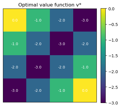
plot_value_heatmap(opt_v, title="Optimal value function v*")
Output:
Optimal policy (arrows):
■ ← ← ↓
↑ ↑ ↑ ↓
↑ ↑ → ↓
↑ → → ■
Output Analysis
-
Optimal value function $v^*$:
Values represent expected cumulative return under the optimal policy. Terminal states have value 0; values decrease by ~1 per step away due to the step cost. -
Optimal policy:
Arrows point toward the nearest terminal, choosing shortest paths and avoiding extra steps. -
Sanity check:
Symmetry in values and actions matches the grid and reward structure, confirming correct convergence of policy iteration.
6. Comparing to “Partial” Policy Iteration
One practical variant is to not fully solve the policy evaluation step each time, but do:
- A fixed number of evaluation sweeps (e.g., 5 or 10 Bellman updates), then
- A greedy improvement step again.
This is sometimes called modified policy iteration and interpolates between:
- Value iteration (1 sweep per improvement), and
- Classical policy iteration (fully evaluate each time).
We’ll do a small experiment with partial evaluation to show it still converges.
Code:
def partial_policy_iteration(P, R, gamma, theta=1e-4,
max_eval_sweeps=5, max_outer_iters=100, verbose=True):
"""
Modified policy iteration:
- Do at most max_eval_sweeps evaluation sweeps per outer loop.
- Then greedy policy improvement.
"""
S, A, _ = P.shape
rng = np.random.default_rng(1)
policy = rng.integers(low=0, high=A, size=S, dtype=int)
for s in TERMINAL_STATES:
policy[s] = 0
v = np.zeros(S, dtype=float)
outer_hist = []
for outer in range(max_outer_iters):
if verbose:
print(f"\n=== Outer iter {outer} ===")
# Partial evaluation
for sweep in range(max_eval_sweeps):
delta = 0.0
v_new = v.copy()
for s in range(S):
if s in TERMINAL_STATES:
continue
a = policy[s]
v_new[s] = R[s, a] + gamma * np.dot(P[s, a], v)
delta = max(delta, abs(v_new[s] - v[s]))
v = v_new
if delta < theta:
if verbose:
print(f" Evaluation converged early at sweep={sweep}, delta={delta:.6g}")
break
outer_hist.append((v.copy(), policy.copy()))
# Improvement
new_policy, stable = greedy_policy_improvement(P, R, gamma, v, policy)
changes = (new_policy != policy).sum()
if verbose:
print(f" Policy changes: {changes}, stable? {stable}")
policy = new_policy
if stable:
if verbose:
print("Modified policy iteration converged.")
break
return policy, v, outer_hist
mpi_policy, mpi_v, mpi_hist = partial_policy_iteration(
P, R, gamma, theta=1e-4, max_eval_sweeps=5, verbose=False
)
print("Modified PI — optimal policy (arrows):")
print_policy(mpi_policy)
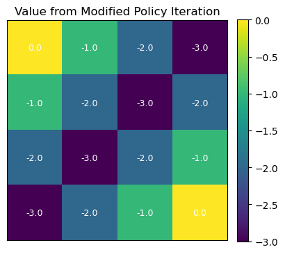
plot_value_heatmap(mpi_v, title="Value from Modified Policy Iteration")
Output:
Modified PI — optimal policy (arrows):
■ ← ← ↓
↑ ↑ ↑ ↓
↑ ↑ → ↓
↑ → → ■
Key Takeaways
- Policy evaluation computes $v_\pi$ for a fixed policy by solving the Bellman expectation equation.
- Policy improvement greedifies w.r.t. $v_\pi$, producing a better (or equal) policy.
- Policy iteration alternates evaluation and improvement and converges to an optimal policy in finite discounted MDPs.
- Implementation is straightforward for tabular MDPs: you need $P$, $R$, and a deterministic policy array.
- Variants like modified policy iteration trade off evaluation accuracy vs. speed and connect policy iteration to value iteration.
Next: 15_dp_value_iteration.ipynb → directly iterating the optimal Bellman operator $v_{k+1} = \max_a T^a v_k$ without an explicit policy evaluation step.