Introduction to Markov Chains
A visual, hands‑on primer with NumPy + Matplotlib
What you’ll learn
- Markov property, transition matrices, and multi‑step transitions
- Simulating Markov chains & visualizing convergence
- Stationary distributions, ergodicity, mixing
- Absorbing chains & absorption probabilities
- Markov Reward Processes (MRPs) and Bellman equations (link to RL)
- Mini PageRank demo
How to use: Read each Theory block, then run the following code cells.
1. Markov Chains — Core Ideas
A discrete-time Markov chain (DTMC) is a sequence of random variables $X_0, X_1, \ldots$ on a finite state space $\mathcal{S} = {1,\dots,n}$ satisfying the Markov property:
\[\Pr[X_{t+1}=j \mid X_t=i, X_{t-1},\dots] \;=\; \Pr[X_{t+1}=j \mid X_t=i] \;=\; P_{ij}.\]The matrix $P \in \mathbb{R}^{n \times n}$ is the transition matrix, where:
- $P_{ij} \ge 0$
- $\sum_j P_{ij} = 1$ (each row is a probability distribution)
- A state distribution is a row vector $\mu \in \Delta^{n-1}$.
-
One-step evolution:
\[\mu_{t+1} = \mu_t P .\]
k-step transitions (Chapman–Kolmogorov):
\[\Pr[X_{t+k}=j \mid X_t=i] = (P^k)_{ij}, \qquad \mu_{t+k} = \mu_t P^k.\]This shows how a Markov chain evolves over time via matrix powers.
Why this matters for RL
In reinforcement learning, an MDP augments Markov chains with actions. For each action $a$, there is a transition matrix $P^a$. A fixed policy $\pi(a \mid s)$ induces a Markov chain over states with:
\[P^\pi = \sum_{a} \Pi_a \, P^a,\]where $\Pi_a = \mathrm{diag}(\pi(a \mid s_1), \ldots, \pi(a \mid s_n))$.
Thus, many RL concepts — stationary distributions, mixing, long-term visitation frequencies, discounted returns — rest directly on Markov chain behavior.
Markov chains are the foundation for understanding value functions, policy evaluation, and the dynamics of exploration in MDPs.
Code:
import numpy as np
import matplotlib.pyplot as plt
# Cleaner printing for matrices
np.set_printoptions(precision=3, suppress=True)
# Transition matrix for a simple 4-state Markov chain
P = np.array([
[0.10, 0.85, 0.05, 0.00], # from state 0
[0.00, 0.15, 0.80, 0.05], # from state 1
[0.05, 0.00, 0.10, 0.85], # from state 2
[0.80, 0.05, 0.00, 0.15], # from state 3
], dtype=float)
# Verify stochasticity (each row should sum to 1)
print("Row sums (should be 1.0):", P.sum(axis=1))
# One-step and multi-step evolution
pi0 = np.array([1.0, 0.0, 0.0, 0.0]) # Start in state 0 with full probability
pi1 = pi0 @ P # distribution after 1 step
pi5 = pi0 @ np.linalg.matrix_power(P, 5) # distribution after 5 steps
pi10 = pi0 @ np.linalg.matrix_power(P, 10) # distribution after 10 steps
pi15 = pi0 @ np.linalg.matrix_power(P, 15) # distribution after 15 steps
pi20 = pi0 @ np.linalg.matrix_power(P, 20) # distribution after 20 steps
print("\nDistribution after 1 step (pi1):", pi1)
print("Distribution after 5 steps (pi5):", pi5)
print("Distribution after 10 steps (pi10):", pi10)
print("Distribution after 15 steps (pi15):", pi15)
print("Distribution after 20 steps (pi20):", pi20)
# Visualize how distributions evolve over time
T = 20
dist = np.zeros((T, 4))
dist[0] = pi0
for t in range(1, T):
dist[t] = dist[t-1] @ P
plt.figure(figsize=(7,4))
for s in range(4):
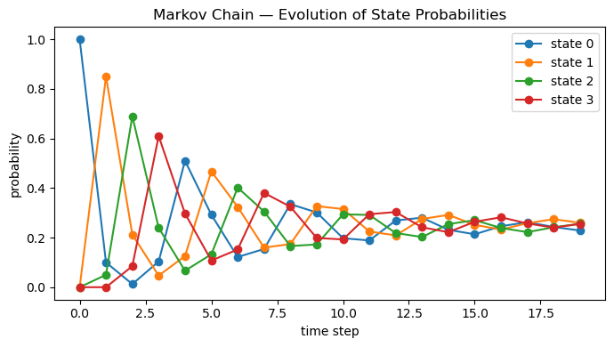
plt.plot(dist[:, s], marker='o', label=f"state {s}")
plt.title("Markov Chain — Evolution of State Probabilities")
plt.xlabel("time step")
plt.ylabel("probability")
plt.legend()
plt.tight_layout()
plt.show()
Output:
    Row sums (should be 1.0): [1. 1. 1. 1.]

    Distribution after 1 step (pi1): [0.1  0.85 0.05 0.  ]
    Distribution after 5 steps (pi5): [0.292 0.467 0.133 0.107]
    Distribution after 10 steps (pi10): [0.198 0.315 0.294 0.193]
    Distribution after 15 steps (pi15): [0.214 0.252 0.27  0.264]
    Distribution after 20 steps (pi20): [0.24  0.246 0.245 0.269]
2. Stationary Distribution & Ergodicity
A distribution $\pi^*$ is stationary for a Markov chain with transition matrix $P$ if:
\[\pi^* = \pi^* P, \qquad \sum_{i} \pi^*_i = 1, \qquad \pi^*_i \ge 0.\]It is a fixed point of the dynamics — once the chain reaches $\pi^*$, it stays there forever.
Ergodicity
A finite Markov chain is ergodic if it is:
- Irreducible (all states communicate), and
- Aperiodic (no deterministic cycles).
For an ergodic chain:
\[\lim_{t \to \infty} \pi_0 P^t = \pi^*,\]meaning all initial distributions converge to the same stationary distribution. This is the long-run behavior of the system.
Computing $\pi^*$
Several equivalent methods:
-
As the left eigenvector of $P$ for eigenvalue 1:
$ \pi^* P = \pi^*. $$
-
Solve the linear system:
\[(I - P^\top)\pi = 0, \qquad \sum_i \pi_i = 1.\] -
Empirically by power iteration: repeatedly apply $P$ to any distribution vector.
RL Connection
In Reinforcement Learning, a policy $\pi(a \mid s)$ induces a Markov chain over states with transition matrix:
\[P^{\pi}(s' \mid s) = \sum_a \pi(a \mid s)\, P(s' \mid s, a).\]Its stationary distribution $d^{\pi}$ describes how often the agent visits each state in the long run.
This distribution directly affects:
- State visitation frequencies (important for exploration),
- Policy gradient estimates (reward expectations weighted by $d^{\pi}$),
- Value function definitions in continuing tasks.
In short: stationary distributions tell us what the agent “sees” most often under a fixed policy.
Code:
# Evolve distribution over time (needed for empirical distribution)
T = 2000
pi = pi0.copy() # from earlier: pi0 = [1,0,0,0]
emp = [pi.copy()]
for _ in range(T):
pi = pi @ P # evolve one step
emp.append(pi.copy())
emp = np.array(emp)
# Stationary distribution via left eigenvector of P
evals, evecs = np.linalg.eig(P.T)
idx = np.argmin(np.abs(evals - 1.0))
v = np.real_if_close(evecs[:, idx])
pi_star = v / v.sum()
pi_star = np.maximum(pi_star, 0); pi_star = pi_star / pi_star.sum()
print("Eigenvalue closest to 1:", evals[idx])
print("Stationary distribution π*:", np.round(pi_star, 6))
# Compare with empirical long-run distribution
emp_last = emp[-1]
print("Empirical (T = {}):".format(len(emp)-1), np.round(emp_last, 6))
print("L1 difference ||π* - empirical||₁:",
float(np.sum(np.abs(pi_star - emp_last))))
# Plot
labels = [f"s{i}" for i in range(P.shape[0])]
x = np.arange(len(labels))
plt.figure(figsize=(6.4,3.6))
plt.bar(x-0.15, pi_star, width=0.3, label="stationary π*")
plt.bar(x+0.15, emp_last, width=0.3, label=f"empirical T={len(emp)-1}")
plt.xticks(x, labels)
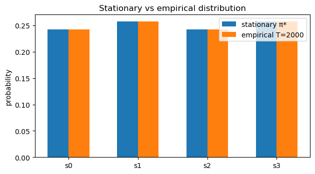
plt.ylabel("probability"); plt.title("Stationary vs empirical distribution")
plt.legend(); plt.tight_layout(); plt.show()
Output:
Eigenvalue closest to 1: (1.000000000000002+0j)
Stationary distribution π*: [0.242 0.258 0.242 0.258]
Empirical (T = 2000): [0.242 0.258 0.242 0.258]
L1 difference ||π* - empirical||₁: 2.942091015256665e-15
3. Absorbing Chains & Absorption Probabilities
A Markov chain is absorbing if it contains at least one absorbing state (i.e., a state $ i $ such that $P_{ii} = 1$) and from any other state there is a path to some absorbing state.
We reorder the states into:
- Transient states $T$
- Absorbing states $A$
so that the transition matrix becomes block-structured:
\[P = \begin{pmatrix} Q & R \\ 0 & I \end{pmatrix},\]where:
- $ Q \in \mathbb{R}^{|T| \times |T|} $ describes transitions among transient states
- $ R \in \mathbb{R}^{|T| \times |A|} $ describes transitions from transient → absorbing
- $ I $ is an identity matrix for absorbing states (they remain where they are)
Fundamental Matrix
The fundamental matrix is:
\[N = (I - Q)^{-1},\]and it encodes the expected number of times the chain visits each transient state before absorption.
Absorption Probabilities
The probability of being absorbed in each absorbing state, starting from each transient state, is:
\[B = N R,\]where $B_{ij}$ is the probability of eventual absorption in absorbing state $j$ given that we start in transient state $i$.
RL Connection
Absorbing chains relate directly to episodic RL:
- Termination states in an MDP correspond to absorbing states
- The matrix $Q$ describes transient transitions before the episode ends
- Absorption probabilities mirror termination likelihoods, relevant for:
- episodic value calculations,
- analyzing horizon lengths,
- proving convergence of TD methods on finite MDPs.
Absorbing MDPs are also the basis of absorbing Markov decision processes, useful in safety-constrained RL and risk analysis.
Code:
# Toy absorbing chain: states 0,1 transient; states 2,3 absorbing
P_abs = np.array([
    [0.5, 0.4, 0.1, 0.0],  # state 0 (transient)
    [0.2, 0.5, 0.0, 0.3],  # state 1 (transient)
    [0.0, 0.0, 1.0, 0.0],  # state 2 (absorbing)
    [0.0, 0.0, 0.0, 1.0],  # state 3 (absorbing)
], dtype=float)

# Partition into Q (transient→transient) and R (transient→absorbing)

Q = P_abs[:2, :2] # states 0,1 → 0,1
R = P_abs[:2, 2:] # states 0,1 → 2,3

I = np.eye(Q.shape[0])

# Fundamental matrix: expected #visits to transient states before absorption
N = np.linalg.inv(I - Q)

# Absorption probabilities: B[i,j] = P(absorbed in j | start in i)
B = N @ R

np.set_printoptions(precision=4, suppress=True)

print("Q (transient→transient):\n", Q)
print("\nR (transient→absorbing):\n", R)
print("\nFundamental matrix N = (I - Q)^(-1):\n", N)
print("\nAbsorption probabilities B = N R:\n", B)

# Each row of B should sum to 1 (eventually absorbed somewhere)
print("\nRow sums of B (should be ~1):", B.sum(axis=1))
Output:
Q (transient→transient):
 [[0.5 0.4]
 [0.2 0.5]]

R (transient→absorbing):
 [[0.1 0. ]
 [0.  0.3]]

Fundamental matrix N = (I - Q)^(-1):
 [[2.9412 2.3529]
 [1.1765 2.9412]]

Absorption probabilities B = N R:
 [[0.2941 0.7059]
 [0.1176 0.8824]]

Row sums of B (should be ~1): [1. 1.]
4. Markov Reward Processes (MRPs) & the Bellman Equation
A Markov Reward Process (MRP) adds rewards and discounting to a Markov chain. Formally, an MRP is a tuple $(\mathcal{S}, P, r, \gamma)$:
- $P$: transition matrix
- $r(s)$: expected immediate reward in state $s$
- $\gamma \in [0,1)$: discount factor
-
Value function:
\[v(s) = \mathbb{E}\left[\sum_{t=0}^\infty \gamma^t R_{t} \mid S_0=s\right]\]
The Bellman equation for MRPs is:
\[v = r + \gamma P v\]This gives a closed-form solution:
\[v = (I - \gamma P)^{-1} r.\]Why this matters for RL
-
In an MDP, picking a policy $\pi(a \mid s)$ induces an MRP with transition matrix:
\[P^\pi = \sum_{a} \pi(a \mid s) P^{a}\] -
Policy evaluation reduces to solving:
\[v^\pi = r^\pi + \gamma P^\pi v^\pi\] - All value-based RL algorithms (TD, Monte Carlo, Dynamic Programming, DQN) are approximations to this equation.
- Understanding MRPs builds intuition for stability, contraction mappings, and why iterative Bellman updates converge.
This section bridges Markov chains → MRPs → full RL.
Code:
# Markov Reward Process (MRP) Evaluation

# Discount and per-state rewards
gamma = 0.95
r = np.array([+1.0, -0.2, +0.3, 0.0], dtype=float)   # reward for each state

# Identity
I = np.eye(P.shape[0])

# Closed-form Bellman solution: v = (I - γP)^(-1) r
A = I - gamma * P
v_closed = np.linalg.solve(A, r)

print("Closed-form value v:", np.round(v_closed, 4))

# Iterative (Dynamic Programming) Policy Evaluation
# v_{k+1} = r + γ P v_k
v_it = np.zeros_like(r)
num_iter = 300

for _ in range(num_iter):
    v_it = r + gamma * (P @ v_it)

print("Iterative value v:", np.round(v_it, 4))

# L∞ difference between iterative and closed-form
err = np.max(np.abs(v_closed - v_it))
print("Max difference:", round(err, 6))
Output:
Closed-form value v: [5.6715 4.8031 5.3517 5.2927]
Iterative value v: [5.6715 4.8031 5.3517 5.2927]
Max difference: 1e-06
5. Mini PageRank (Random Surfer Model)
PageRank models a random surfer on a directed graph. If a webpage has outgoing links, the surfer follows one at random; otherwise, they teleport uniformly.
Given a link matrix $S$ (row-stochastic) and damping factor $\alpha \in (0,1)$, the Google transition matrix is:
\[P_{\alpha} \;=\; \alpha S \;+\; (1-\alpha)\frac{1}{n}\mathbf{1}\mathbf{1}^\top,\]where:
- $ \alpha \approx 0.85 $ is the probability of following a real link.
- $ (1-\alpha) $ is the probability of teleportation to any page.
- $n$ is the number of nodes.
The PageRank vector $ \pi^* $ is the stationary distribution:
\[\pi^* = \pi^* P_{\alpha}, \quad \sum_i \pi^*_i = 1.\]Because $P_\alpha$ is irreducible and aperiodic, it has a unique stationary distribution, and power iteration converges rapidly.
RL Connection
PageRank is mathematically identical to evaluating the value distribution of a random policy in an MDP with:
- teleportation → exploration bonus,
- link structure → transition probabilities.
This mirrors entropy-regularized RL and stochastic policies where transitions combine structured dynamics with exploration.
Code:
np.set_printoptions(precision=4, suppress=True)
A = np.array([
[0, 1, 1, 0], # 0 -> 1,2
[0, 0, 1, 1], # 1 -> 2,3
[1, 0, 0, 1], # 2 -> 0,3
[1, 0, 0, 0], # 3 -> 0
], dtype=float)
n = A.shape[0]
# Build S: row-stochastic link matrix
S = A.copy()
row_sums = S.sum(axis=1, keepdims=True)
for i in range(n):
if row_sums[i, 0] > 0: # non-dangling row → normalize
S[i, :] /= row_sums[i, 0]
else: # dangling row → uniform
S[i, :] = 1.0 / n
print("Link matrix S:")
print(S)
print("Row sums S:", S.sum(axis=1))
# Google matrix P_pr
alpha = 0.85
teleport = np.ones((n, n)) / n
P_pr = alpha * S + (1 - alpha) * teleport
print("\nGoogle matrix P_pr:")
print(P_pr)
print("Row sums P_pr:", P_pr.sum(axis=1))
# PageRank as stationary distribution of P_pr
evals, evecs = np.linalg.eig(P_pr.T)
idx = np.argmin(np.abs(evals - 1.0))
v = np.real_if_close(evecs[:, idx])
pr = v / v.sum()
pr = np.maximum(pr, 0.0)
pr = pr / pr.sum()
print("\nEigenvalue closest to 1:", evals[idx])
print("PageRank π*:", np.round(pr, 4), " sum:", pr.sum())
# Plot
labels = [f"node {i}" for i in range(n)]
x = np.arange(n)
plt.figure(figsize=(5.6, 3.6))
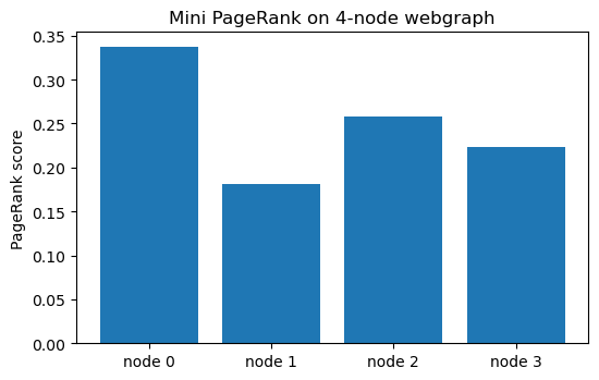
plt.bar(x, pr)
plt.xticks(x, labels)
plt.ylabel("PageRank score")
plt.title("Mini PageRank on 4-node webgraph")
plt.tight_layout()
plt.show()
Output:
Link matrix S:
[[0.  0.5 0.5 0. ]
 [0.  0.  0.5 0.5]
 [0.5 0.  0.  0.5]
 [1.  0.  0.  0. ]]
Row sums S: [1. 1. 1. 1.]

Google matrix P_pr:
[[0.0375 0.4625 0.4625 0.0375]
 [0.0375 0.0375 0.4625 0.4625]
 [0.4625 0.0375 0.0375 0.4625]
 [0.8875 0.0375 0.0375 0.0375]]
Row sums P_pr: [1. 1. 1. 1.]

Eigenvalue closest to 1: (1.0000000000000009+0j)
PageRank π*: [0.3374 0.1809 0.2578 0.2239]  sum: 1.0
Key Takeaways
- Markov chain dynamics: Distributions evolve by multiplication with the transition matrix $\pi_{t+1} = \pi_t P$, and multi-step transitions follow $P^k$.
- Stationary distributions: For an ergodic chain, all initial distributions converge to the unique long-run distribution $\pi^*$.
- Absorbing chains: Transient–absorbing structure leads to closed-form absorption probabilities via the fundamental matrix $N=(I-Q)^{-1}$.
- Markov Reward Processes (MRPs): Adding rewards and discount yields value functions solving the Bellman equation $v = r + \gamma P v$.
- Policies induce chains: In an MDP, fixing a policy $\pi(a \mid s)$ produces a Markov chain with transition matrix $P^\pi$, laying the foundation for prediction and control in RL.
Next: Although the logical next step is Phase 1 — Fundamentals (MDPs, Bellman equations, Dynamic Programming, Monte Carlo, TD learning), it’s highly recommended to solidify Phase 0 foundations first through hands-on mini-projects.
Start with 09_linear_regression_project.ipynb to reinforce key ML and numerical concepts before diving into full RL.