Agent–Environment Interaction
How agents and environments talk to each other in RL.
What you’ll learn
- The agent–environment loop: how actions, states, and rewards evolve over time.
- The structure of a trajectory $ (S_0, A_0, R_1, S_1, \dots) $.
- Episodic vs continuing tasks and how we define returns.
- Discounted return $ G_t $ and why discounting matters.
- A tiny bandit environment to simulate interaction and visualize returns.
This notebook sets the conceptual foundation for everything in RL: MDPs, Bellman equations, DP, Monte Carlo, TD, and beyond.
Code:
import numpy as np
import matplotlib.pyplot as plt

np.set_printoptions(precision=3, suppress=True)

# For reproducibility
rng = np.random.default_rng(0)

def plot_series(values, title, xlabel="t", ylabel="value"):
    plt.figure(figsize=(6.4, 3.6))
    plt.plot(values, marker="o", alpha=0.8)
    plt.title(title)
    plt.xlabel(xlabel)
    plt.ylabel(ylabel)
    plt.tight_layout()
    plt.show()
1. The Agent–Environment Loop
In reinforcement learning, we model interaction as a repeated loop between:
- the agent (the learner/decision-maker), and
- the environment (everything else).
At each discrete time step $ t = 0, 1, 2, \dots $:
- The agent observes a state $ S_t $.
-
The agent selects an action $ A_t $ according to its policy $ \pi $:
\[A_t \sim \pi(\cdot \mid S_t).\] - The environment responds with:
- a reward $ R_{t+1} $,
- the next state $ S_{t+1} $.
This yields a trajectory:
\[S_0, A_0, R_1, S_1, A_1, R_2, S_2, \dots\]The agent’s goal is to choose actions to maximize some notion of cumulative reward over time.
Episodic vs Continuing Tasks
-
Episodic tasks: interaction breaks into episodes
\[S_0, A_0, R_1, \dots, S_T\]where $ T $ is a (random) terminal time.
-
Continuing tasks: interaction goes on indefinitely with no terminal state.
In both cases, we will soon define a return $ G_t $ that aggregates rewards into a scalar objective.
RL Connection
This loop is the backbone of everything in RL:
- Dynamic Programming, Monte Carlo, and TD all estimate value functions based on the sequence $ (S_t, A_t, R_{t+1}) $.
- Policy Gradient and Actor–Critic methods adjust the policy $ \pi(a \mid s) $ using information from these trajectories.
- Environments like Gymnasium implement this loop via
reset()andstep()calls.

2. Multi-Armed Bandits — The Simplest RL Environment
Before building any environment, let’s establish terminology.
A k-armed bandit is the simplest form of reinforcement learning:
- The agent chooses an action (arm) $ a \in {0,1,\dots,k-1} $.
- The environment returns a reward $ R_{t+1} $ drawn from an unknown distribution with true mean $ \mu_a $.
- There is no state and no transition — every step is independent.
Formally, at each step:
\[A_t \sim \pi(a), \qquad R_{t+1} \sim \mathcal{D}_a.\]This is an MDP with:
- 1 state,
- k actions,
- reward distribution $ R(a) $,
- no episode termination (continuing task).
Why start with bandits?
They highlight:
- exploration vs exploitation
- value estimation
- stochastic rewards
- incremental updates
- policies as distributions over actions
These concepts form the backbone of RL algorithms like SARSA, Q-learning, REINFORCE, and actor–critic.
RL Connection
Bandits = the “hello world” of RL.
They strip away transitions and dynamics so we can focus on:
- action selection,
- reward estimation,
- policy improvement.
Next, we will create a minimal bandit environment class to simulate the agent–environment loop.
Code:
class KArmedBandit:
    """
    Simple k-armed bandit:
    - Agent chooses action a ∈ {0,...,k-1}
    - Reward ~ Normal(mean[a], noise_std)
    - No state, no termination
    """
    def __init__(self, means, noise_std=0.1, rng=None):
        self.means = np.array(means, dtype=float)
        self.k = len(means)
        self.noise_std = noise_std
        self.rng = rng if rng is not None else np.random.default_rng()

    def reset(self):
        return None, {}

    def step(self, action):
        assert 0 <= action < self.k
        true_mean = self.means[action]
        reward = float(self.rng.normal(true_mean, self.noise_std))
        return None, reward, False, False, {"true_mean": true_mean}

bandit = KArmedBandit(means=[0.2, 0.0, -0.1], noise_std=0.1)

for a in range(3):
    _, r, _, _, info = bandit.step(a)
    print(f"Action {a} → reward {r:.3f}, true mean={info['true_mean']}")
Output:
Action 0 → reward 0.172, true mean=0.2
Action 1 → reward -0.106, true mean=0.0
Action 2 → reward -0.141, true mean=-0.1
3. Trajectories & Discounted Return
To measure long-term performance, we define the return at time $ t $ as the sum of future rewards.
Episodic Return
For an episode that terminates at time $ T $, the undiscounted return from time $ t $ is:
\[G_t = \sum_{k=0}^{T-t-1} R_{t+1+k}.\]Discounted Return
Often we prefer discounted returns to:
- prioritize near-term rewards,
- guarantee convergence for infinite horizons, and
- model uncertainty in the future.
For discount factor $ \gamma \in [0,1) $:
\[G_t = \sum_{k=0}^{\infty} \gamma^k R_{t+1+k}.\]- If $ \gamma \approx 0 $: myopic, cares mainly about immediate reward.
- If $ \gamma \approx 1 $: far-sighted, cares about long-term consequences.
RL Connection
- Value functions estimate expected return $ v_\pi(s) = \mathbb{E}_\pi[G_t \mid S_t = s] $.
- Bellman equations, DP, MC, and TD all revolve around different ways of estimating $ G_t $ or its expectation.
We’ll now simulate returns for a random policy interacting with our bandit.
Code:
def random_policy(k):
"""Uniform random policy over k actions."""
return rng.integers(low=0, high=k)
def run_bandit_episodes(env, policy_fn, n_episodes=25, horizon=10, gamma=0.9):
"""
Simulate n_episodes of length 'horizon' with discount γ.
Returns:
- returns: list of total discounted returns per episode
- rewards_per_ep: list of list of per-step rewards
"""
all_returns = []
all_rewards = []
for ep in range(n_episodes):
obs, info = env.reset()
rewards = []
for t in range(horizon):
a = policy_fn(env.k)
obs, r, term, trunc, info = env.step(a)
rewards.append(r)
# compute discounted return G_0 for this episode
G = 0.0
for t, r in enumerate(rewards):
G += (gamma**t) * r
all_returns.append(G)
all_rewards.append(rewards)
return np.array(all_returns), all_rewards
gamma = 0.9
returns, rewards_per_ep = run_bandit_episodes(
bandit, random_policy, n_episodes=25, horizon=20, gamma=gamma
)
print("Mean discounted return (random policy):", np.round(returns.mean(), 3))
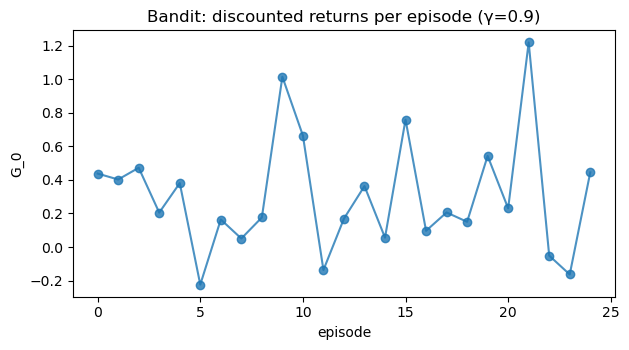
plot_series(returns, title=f"Bandit: discounted returns per episode (γ={gamma})",
xlabel="episode", ylabel="G_0")
Output:
Mean discounted return (random policy): 0.305
4. Policies as Probability Distributions
A policy $ \pi $ describes how the agent selects actions:
- Deterministic: $ \pi(s) = a $ (a single action per state), or
- Stochastic: $ \pi(a \mid s) = \Pr[A_t = a \mid S_t = s] $.
In the bandit case (no state), the policy reduces to a distribution over actions $ \pi(a) $.
We want to learn a policy that prefers arms with higher reward.
A simple approach for bandits:
- Maintain sample-average estimates $ \hat{Q}_t(a) $ of each arm’s value.
- Select actions via $\varepsilon$-greedy:
- with probability $ \varepsilon $: explore (random arm),
- with probability $ 1 - \varepsilon $: exploit $ \arg\max_a \hat{Q}_t(a) $.
This is a tiny instance of the exploration–exploitation trade-off that appears everywhere in RL.
Code:
def run_eps_greedy_bandit(env, eps=0.1, steps=500):
k = env.k
Q = np.zeros(k) # value estimates
N = np.zeros(k) # counts
rewards = []
obs, info = env.reset()
for t in range(steps):
# ε-greedy action selection
if rng.random() < eps:
a = rng.integers(low=0, high=k)
else:
a = int(np.argmax(Q))
obs, r, term, trunc, info = env.step(a)
rewards.append(r)
# Incremental sample-average update for Q(a)
N[a] += 1
Q[a] += (r - Q[a]) / N[a]
return np.array(rewards), Q, N
steps = 500
rewards_eps01, Q_eps01, N_eps01 = run_eps_greedy_bandit(bandit, eps=0.1, steps=steps)
rewards_eps0, Q_eps0, N_eps0 = run_eps_greedy_bandit(bandit, eps=0.0, steps=steps) # purely greedy
print("True means:", bandit.means)
print("ε=0.1 estimates Q:", np.round(Q_eps01, 3))
print("ε=0.0 estimates Q:", np.round(Q_eps0, 3))
# Compare average reward over time
def running_mean(x, window=20):
x = np.asarray(x)
if len(x) < window:
return x
kernel = np.ones(window) / window
return np.convolve(x, kernel, mode="valid")
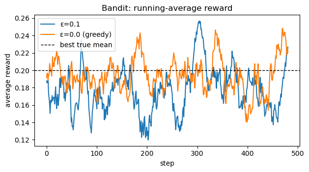
plt.figure(figsize=(6.4, 3.6))
plt.plot(running_mean(rewards_eps01), label="ε=0.1")
plt.plot(running_mean(rewards_eps0), label="ε=0.0 (greedy)")
plt.axhline(np.max(bandit.means), color="k", linestyle="--", linewidth=1, label="best true mean")
plt.title("Bandit: running-average reward")
plt.xlabel("step")
plt.ylabel("average reward")
plt.legend()
plt.tight_layout()
plt.show()
Output:
True means: [ 0.2  0.  -0.1]
ε=0.1 estimates Q: [ 0.199 -0.015 -0.091]
ε=0.0 estimates Q: [0.194 0.    0.   ]
4. Markov Property & MDP Preview
So far, our environment had no state. In full RL problems, we typically assume the Markov property:
\[\Pr[S_{t+1} = s', R_{t+1} = r \mid S_0, A_0, \dots, S_t, A_t] = \Pr[S_{t+1} = s', R_{t+1} = r \mid S_t, A_t].\]That is, the future depends only on the present state and action, not the entire history.
This leads directly to Markov Decision Processes (MDPs):
- State space $ \mathcal{S} $
- Action space $ \mathcal{A} $
- Transition dynamics $ p(s’, r \mid s, a) $
- Discount factor $ \gamma $
- Reward function $ r(s,a) $ or $ r(s,a,s’) $
In the next notebooks, we will:
- Formalize MDPs,
- Define value functions $ v_\pi(s), q_\pi(s,a) $,
- Derive Bellman equations, and
- Use Dynamic Programming, Monte Carlo, and TD to estimate and improve policies.
The simple bandit you just saw is the “state-free” special case of an MDP.
Key Takeaways
-
The agent–environment loop generates trajectories
\[S_0, A_0, R_1, S_1, \dots\]which drive learning in RL.
- Returns aggregate future rewards; discounting with $ \gamma $ balances short- vs long-term objectives.
- A policy $ \pi(a \mid s) $ maps states to action distributions; even in bandits, exploration (ε-greedy) is crucial.
- Bandits are the simplest RL setting and a special case of MDPs with no state.
- This notebook’s bandit examples are a gentle prelude to full Markov Decision Processes and value functions.
Next: 11_markov_decision_processes.ipynb → Formal definition of MDPs, Markov property, transition dynamics, and trajectory distributions.