Gymnasium Basics
Explore the foundation of Reinforcement Learning environments and agent–environment interaction.
What you’ll learn
- The Gymnasium API:
obs, info = env.reset()→obs, reward, terminated, truncated, info = env.step(action) - Handling episode endings:
done = terminated or truncated - Implementing a simple random agent baseline and visualizing episode returns
- A minimal tabular value estimation example to link dynamics with learning
This notebook bridges theory and practice — you’ll interact with environments, collect experience, and prepare for training real RL agents.
Code:
import numpy as np
import matplotlib.pyplot as plt

try:
    import gymnasium as gym
except Exception as e:
    print("Gymnasium not found. Install with: pip install gymnasium gymnasium[classic-control]")
    raise
1. Environment Anatomy
In reinforcement learning, an environment defines the world in which an agent operates. At each time step $ t $, the agent observes a state $ s_t $, takes an action $ a_t $, and receives a reward $ r_t $ while the environment transitions to a new state $ s_{t+1} $:
\[(s_t, a_t, r_t, s_{t+1}) \sim \mathcal{E}\]The standard Gymnasium interface provides two key methods:
env.reset()→ initializes the environment and returns the starting observation.env.step(action)→ applies the chosen action and returns(next_obs, reward, terminated, truncated, info).
An episode ends when terminated (goal reached/failure) or truncated (time limit) is True. The agent’s goal is to maximize the expected return:
In RL practice:
- The environment models the dynamics $ P(s_{t+1} \mid s_t, a_t) $.
- The agent learns a policy $ \pi(a_t \mid s_t) $ that maps observations to actions.
- Tools like Gymnasium provide standard benchmarks (CartPole, MountainCar, etc.) to evaluate and visualize how well the agent learns to act through interaction.
Code:
import gymnasium as gym
import numpy as np

# Create the environment and reset it
env = gym.make("CartPole-v1")
obs, info = env.reset(seed=0)

# Show basic environment details
print("Environment details:")
print(f"Action space: {env.action_space}")
print(f"Observation space: {env.observation_space}")
print(f"Max episode steps: {env.spec.max_episode_steps}")

print(f"\nInitial observation shape: {np.array(obs).shape}")
print(f"Observation sample: {obs}")
print(f"Info dictionary keys: {list(info.keys())}")
Output:
Environment details:
Action space: Discrete(2)
Observation space: Box([-4.8000002e+00 -3.4028235e+38 -4.1887903e-01 -3.4028235e+38], [4.8000002e+00
3.4028235e+38 4.1887903e-01 3.4028235e+38], (4,), float32)
Max episode steps: 500

Initial observation shape: (4,)
Observation sample: [ 0.01369617 -0.02302133 -0.04590265 -0.04834723]
Info dictionary keys: []
2. Random Policy Baseline
Before training a smart agent, it’s important to establish a baseline — how well does an untrained, random policy perform?
A policy $ \pi(a \mid s) $ defines how the agent selects actions given the current state. A random policy simply samples actions uniformly from the action space:
\[a_t \sim \text{Uniform}(\mathcal{A})\]We can then run several episodes to measure the return (total reward per episode):
\[G = \sum_{t=0}^{T} r_t\]This provides a useful benchmark for later comparison — a trained agent should outperform the random baseline by achieving higher average returns.
In reinforcement learning, such baselines are critical for debugging:
- They verify the environment setup and reward signals.
- They help visualize the stochastic dynamics of the task.
- They serve as a lower bound on performance before learning begins.
Code:
def run_random_episode(env, render=False, max_steps=1000, seed=None):
"""Run one episode with a random policy and return total reward."""
obs, info = env.reset(seed=seed)
total_reward = 0.0
for _ in range(max_steps):
action = env.action_space.sample() # random action
obs, reward, terminated, truncated, info = env.step(action)
total_reward += reward
if render:
env.render()
if terminated or truncated:
break
return total_reward
# Run multiple episodes
num_episodes = 25
returns = [run_random_episode(env, seed=i) for i in range(num_episodes)]
print(f"Random policy — mean return: {np.mean(returns):.2f}")
print(f"Min: {np.min(returns):.2f}, Max: {np.max(returns):.2f}")
# Plot episode returns
plt.figure(figsize=(6, 3.5))
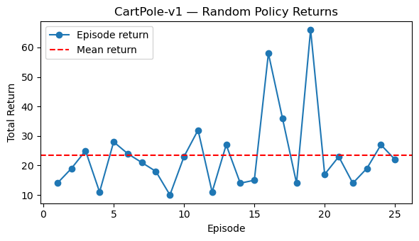
plt.plot(range(1, num_episodes + 1), returns, marker="o", label="Episode return")
plt.axhline(np.mean(returns), color="red", linestyle="--", label="Mean return")
plt.title("CartPole-v1 — Random Policy Returns")
plt.xlabel("Episode")
plt.ylabel("Total Return")
plt.legend()
plt.tight_layout()
plt.show()
Output:
Random policy — mean return: 23.52
Min: 10.00, Max: 66.00
3. Simple Tabular Value Illustration (Toy)
In reinforcement learning, we often estimate the value of taking an action in a given state. For discrete (tabular) environments, this is represented by a Q-table:
\[Q(s, a) \approx \mathbb{E}[R_t + \gamma \max_{a'} Q(s', a')]\]where:
- $ s $ is the current state,
- $ a $ is an action,
- $ R_t $ is the reward received,
- $ s’ $ is the next state, and
- $ \gamma \in [0,1) $ is the discount factor controlling future reward importance.
In continuous environments (like CartPole), we can’t store all states explicitly. So here, we discretize the observation space into coarse bins to approximate a tabular setting. We’ll then use a bandit-like update to tweak action preferences based on received rewards:
This toy example is not a full RL algorithm — it only demonstrates how an agent can incrementally adjust its expectations based on experience.
RL Connection:
- This forms the conceptual bridge between bandits → tabular Q-learning → deep RL.
- Reinforcement learning generalizes this idea by using bootstrapping, discounted returns, and function approximation.
Code:
from collections import defaultdict, deque
n_actions = env.action_space.n
# Coarse discretization bins for 4-D observation
# [cart position, cart velocity, pole angle, pole angular velocity]
bins = [
np.linspace(-4.8, 4.8, 7), # 6 intervals
np.linspace(-3.0, 3.0, 7),
np.linspace(-0.418, 0.418, 7),
np.linspace(-3.5, 3.5, 7),
]
def discretize(obs):
"""Map continuous obs -> tuple of bin indices (tabular key)."""
idxs = []
for o, b in zip(obs, bins):
# clip before binning to avoid out-of-range indices
o = float(np.clip(o, b.min(), b.max()))
idxs.append(int(np.digitize(o, b) - 1)) # indices in [0, len(b)-1]
return tuple(idxs)
# Softmax policy over tabular preferences
prefs = defaultdict(lambda: np.zeros(n_actions, dtype=np.float32))
def softmax(logits, tau=1.0):
z = (logits - np.max(logits)) / max(tau, 1e-6)
ez = np.exp(z, dtype=np.float64)
return (ez / ez.sum()).astype(np.float32)
def run_episode_softmax(env, alpha=0.02, tau=0.8, max_steps=500, baseline=None):
"""One episode of softmax preference learning with immediate-reward update (bandit-like)."""
obs, _ = env.reset()
total = 0.0
for _ in range(max_steps):
s = discretize(obs)
pi = softmax(prefs[s], tau=tau)
a = np.random.choice(n_actions, p=pi)
obs2, r, terminated, truncated, _ = env.step(a)
total += r
# Variance-reduced immediate reward (optional baseline)
adv = r - (baseline if baseline is not None else 0.0)
# REINFORCE-style grad for softmax prefs at state s
grad = -pi
grad[a] += 1.0
# Update preferences
prefs[s] += alpha * adv * grad
# Small clip to keep prefs numerically tame
prefs[s] = np.clip(prefs[s], -20.0, 20.0)
obs = obs2
if terminated or truncated:
break
return total
# Train for multiple episodes
episodes = 150
returns = []
ma = deque(maxlen=10)
for ep in range(episodes):
# Use moving-average reward as a simple baseline
baseline = np.mean(ma) if len(ma) > 0 else None
ret = run_episode_softmax(env, alpha=0.02, tau=0.8, max_steps=500, baseline=baseline)
returns.append(ret)
ma.append(ret)
print(f"Random-ish softmax toy — mean return over {episodes} eps: {np.mean(returns):.2f}")
print(f"Last-10 mean: {np.mean(returns[-10:]):.2f}, max: {np.max(returns):.2f}")
# Plot learning curve
plt.figure(figsize=(6.2, 3.6))
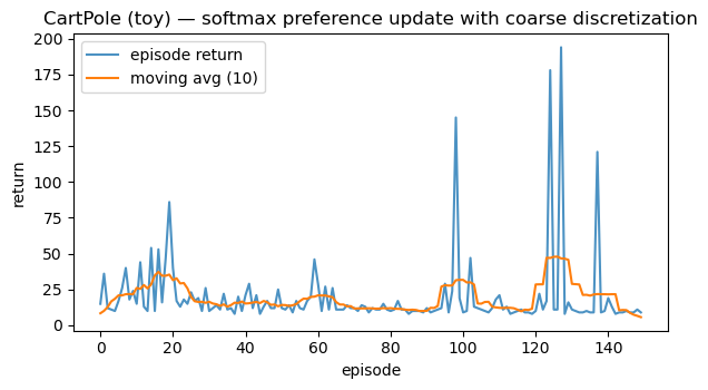
plt.plot(returns, color="tab:blue", alpha=0.8, label="episode return")
# 10-ep moving average
if len(returns) >= 10:
ma_curve = np.convolve(returns, np.ones(10)/10, mode="same")
plt.plot(ma_curve, color="tab:orange", label="moving avg (10)")
plt.title("CartPole (toy) — softmax preference update with coarse discretization")
plt.xlabel("episode"); plt.ylabel("return"); plt.legend()
plt.tight_layout(); plt.show()
env.close()
Output:
Random-ish softmax toy — mean return over 150 eps: 19.61
Last-10 mean: 10.60, max: 194.00
Key Takeaways
- Unified Env API — Gymnasium standardizes
reset()/step()so agents interact consistently across environments. - Random Baseline — Establishes a starting benchmark and reveals environment dynamics early.
- From Tabular to Deep RL — Simple discrete policies expose reward patterns before scaling to neural agents (DQN, PPO, etc.).
Next: 06_basic_machine_learning.ipynb → foundational ML concepts—regression, classification, and evaluation metrics for building RL critics and reward models.