Dynamic Programming: Value Iteration
A from-scratch walkthrough of the Bellman optimality backup to compute $v^$ and an optimal policy.*
What you’ll learn
- How value iteration applies the Bellman optimality operator
- Convergence + stopping criteria ($\theta$) and the role of $\gamma$
- Extracting an optimal greedy policy from $v$
- Visualizing $v$, $\Delta$ (max update), and the learned policy
We’ll use a small GridWorld so everything is transparent and implementable from scratch.
1. Value Iteration — Core Idea
Value Iteration computes the optimal value function by repeatedly applying the Bellman optimality backup:
\[v_{k+1}(s) \;=\; \max_{a} \sum_{s'} P(s' \mid s,a)\Big( r(s,a,s') + \gamma\, v_k(s') \Big)\]At each iteration:
- We assume the agent will act optimally from the next state onward.
- For every state, we evaluate all possible actions and keep the one with the highest expected return.
- Policy improvement is implicit, the greedy policy w.r.t. $v_k$ improves automatically.
Unlike policy evaluation, which evaluates a fixed policy, value iteration merges evaluation and improvement into a single loop.
Why Value Iteration Converges
The Bellman optimality operator is a $\gamma$-contraction (for $\gamma \in [0,1)$):
- Each update shrinks the distance to the optimal value function by at least a factor of $\gamma$.
- This guarantees convergence to a unique fixed point $v^*$, independent of initialization.
Intuitively, future rewards are discounted, so repeated backups eventually stabilize.
RL Connection
- Value iteration is the idealized planning algorithm for known MDPs.
- Q-learning, SARSA, and TD control approximate this same backup using samples instead of full transition models.
- In deep RL, the tabular value $v(s)$ is replaced by a neural network, but the training target still mirrors this Bellman optimality equation.
Value iteration is the conceptual bridge between classical dynamic programming and modern reinforcement learning.
Code:
import numpy as np
import matplotlib.pyplot as plt

np.set_printoptions(precision=3, suppress=True)

# Helper: pretty arrows for policy visualization
ARROWS = {0:"↑", 1:"→", 2:"↓", 3:"←"}  # actions: 0=Up, 1=Right, 2=Down, 3=Left
2. A Simple GridWorld MDP
We use a 4 x 4 grid with:
- Two terminal states: top-left and bottom-right
- Deterministic transitions (attempted moves that hit a wall keep you in place)
- Per-step reward $r=-1$ until termination
- Discount $\gamma$
This is a “shortest path under step penalty” setting where the optimal policy moves toward a terminal in as few steps as possible.
Code:
H, W = 4, 4
nS = H * W  # number of states
nA = 4      # actions: Up, Right, Down, Left

# Action mapping for readability
ARROWS = {0: "↑", 1: "→", 2: "↓", 3: "←"}

# Terminal states: top-left (0,0) and bottom-right (3,3)
terminals = {0, nS - 1}

def to_rc(s):
    """State index -> (row, col)"""
    return divmod(s, W)

def to_s(r, c):
    """(row, col) -> state index"""
    return r * W + c

def step(s, a):
    """
    Deterministic transition function.
    Returns: next_state, reward, done
    """
    # Terminal states are absorbing
    if s in terminals:
        return s, 0.0, True

    r, c = to_rc(s)

    # Proposed move
    if a == 0:    # Up
        r2, c2 = r - 1, c
    elif a == 1:  # Right
        r2, c2 = r, c + 1
    elif a == 2:  # Down
        r2, c2 = r + 1, c
    else:         # Left
        r2, c2 = r, c - 1

    # Wall check: stay in place if outside grid
    if r2 < 0 or r2 >= H or c2 < 0 or c2 >= W:
        s2 = s
    else:
        s2 = to_s(r2, c2)

    done = (s2 in terminals)
    reward = 0.0 if done else -1.0

    return s2, reward, done

# Sanity check: transitions from state 1
print("Transitions from state 1:")
for a in range(nA):
    print(f"  action {ARROWS[a]} ->", step(1, a))
Output:
Transitions from state 1:
  action ↑ -> (1, -1.0, False)
  action → -> (2, -1.0, False)
  action ↓ -> (5, -1.0, False)
  action ← -> (0, 0.0, True)
3. Implementing Value Iteration
Value iteration alternates between estimating how good each state is and improving decisions using the Bellman optimality principle.
Update rule (Bellman optimality backup)
At each iteration, we update every state by assuming we act optimally from the next step onward:
\[v_{k+1}(s) \;=\; \max_a \sum_{s'} P(s' \mid s,a) \big( r(s,a,s') + \gamma\, v_k(s') \big)\]This differs from policy evaluation:
- Policy evaluation: expectation under a fixed policy
- Value iteration: maximization over actions at every update
So improvement and evaluation happen simultaneously.
Stopping criterion
We repeat updates until the values stop changing significantly:
\[\Delta_k = \max_s \big| v_{k+1}(s) - v_k(s) \big|\]When $\Delta_k < \theta$, we declare convergence.
Why this works:
- The Bellman optimality operator is a $\gamma$-contraction
- Repeated application converges to a unique fixed point $v^*$
Extracting the optimal policy
Once the optimal value function $v^*$ is found, the optimal policy is obtained greedily:
\[\pi^*(s) \;\in\; \arg\max_a \sum_{s'} P(s' \mid s,a) \big( r(s,a,s') + \gamma\, v^*(s') \big)\]This step simply asks:
“Given the optimal values, which action is best in each state?”
Intuition
- Value iteration pushes information backward from terminal states
- Each update improves estimates of how far a state is from termination
- In GridWorld, values become negative distances to the nearest terminal
- The resulting policy always moves along the shortest path
Understanding value iteration means understanding the core logic behind almost all RL control algorithms.
Code:
def value_iteration(gamma=0.95, theta=1e-10, max_iters=10_000):
    """
    Synchronous Value Iteration:
      v_{k+1}(s) = max_a [ r(s,a,s') + gamma * v_k(s') ]
    """
    v = np.zeros(nS, dtype=float)
    deltas = []

    for it in range(max_iters):
        v_new = v.copy()
        delta = 0.0

        for s in range(nS):
            if s in terminals:
                v_new[s] = 0.0
                continue

            # Bellman optimality backup (deterministic transitions here)
            q_sa = np.empty(nA, dtype=float)
            for a in range(nA):
                s2, r, done = step(s, a)
                q_sa[a] = r + gamma * v[s2]  # use OLD v (synchronous)

            v_new[s] = np.max(q_sa)
            delta = max(delta, abs(v_new[s] - v[s]))

        v = v_new
        deltas.append(delta)

        if delta < theta:
            break

    return v, np.array(deltas)


def greedy_policy_from_v(v, gamma=0.95, tie_break="first"):
    """
    Extract greedy policy:
      pi(s) = argmax_a [ r + gamma * v(s') ]
    tie_break:
      - "first": np.argmax (first max)
      - "random": random among ties (useful in symmetric grids)
    """
    pi = np.full(nS, -1, dtype=int)
    rng = np.random.default_rng(0)

    for s in range(nS):
        if s in terminals:
            pi[s] = -1
            continue

        q_sa = np.empty(nA, dtype=float)
        for a in range(nA):
            s2, r, done = step(s, a)
            q_sa[a] = r + gamma * v[s2]

        if tie_break == "random":
            best = np.flatnonzero(q_sa == q_sa.max())
            pi[s] = int(rng.choice(best))
        else:
            pi[s] = int(np.argmax(q_sa))

    return pi


# Run
gamma = 0.95
v_star, deltas = value_iteration(gamma=gamma, theta=1e-10, max_iters=10_000)
pi_star = greedy_policy_from_v(v_star, gamma=gamma, tie_break="first")

print("Iterations:", len(deltas))
print("Final max Δ:", deltas[-1] if len(deltas) else None)
print("v* reshape:\n", np.round(v_star.reshape(H, W), 3))
Output:
Iterations: 3
Final max Δ: 0.0
v* reshape:
 [[ 0.    0.   -1.   -1.95]
 [ 0.   -1.   -1.95 -1.  ]
 [-1.   -1.95 -1.    0.  ]
 [-1.95 -1.    0.    0.  ]]
4. Visualizing the Optimal Value Function and Policy
To better understand the result of value iteration, we visualize three key artifacts:
-
Optimal value function $v^*$
Displayed as a heatmap over the grid, where brighter cells indicate higher expected return. This shows how “good” each state is under optimal behavior. -
Greedy policy $\pi^*$ induced by $v^*$
Each arrow indicates the action that maximizes the Bellman optimality backup at that state. Terminal states are marked with ■ since no action is taken there. -
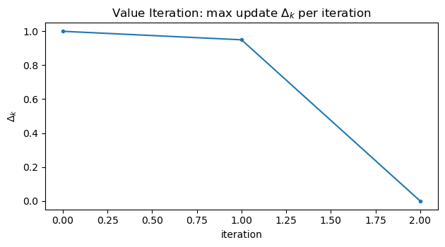
Convergence diagnostics
\[\Delta_k = \max_s |v_{k+1}(s) - v_k(s)|\]
We plot the maximum Bellman update changeto confirm contraction and convergence to the fixed point.
Together, these plots provide:
- geometric intuition for shortest-path behavior,
- a sanity check that the policy points toward terminal states,
- and empirical evidence that value iteration converges as theory predicts.
Code:
def plot_values_and_policy(v, pi, deltas=None, title="Value Iteration", overlay_policy=True):
    """
    Visualize:
      1) Heatmap of v* with numeric annotations
      2) Greedy policy as arrows (printed + optionally overlayed)
      3) Convergence curve of deltas (if provided)
    """
    V = v.reshape(H, W)

    # 1) Heatmap of values
    plt.figure(figsize=(5.6, 4.8))
    im = plt.imshow(V, aspect="equal", origin="upper")
    plt.colorbar(im, fraction=0.046, pad=0.04)
    plt.title(f"{title}: optimal value function $v^*$")
    plt.xticks([]); plt.yticks([])

    vmin, vmax = np.min(V), np.max(V)
    mid = 0.5 * (vmin + vmax)

    for r in range(H):
        for c in range(W):
            s = to_s(r, c)
            if s in terminals:
                txt = "■"
            else:
                txt = f"{V[r, c]:.1f}"

            color = "black" if V[r, c] > mid else "white"
            plt.text(c, r, txt, ha="center", va="center", color=color, fontsize=10, fontweight="bold")

    if overlay_policy:
        for r in range(H):
            for c in range(W):
                s = to_s(r, c)
                if s in terminals:
                    continue
                plt.text(c, r + 0.32, ARROWS[pi[s]], ha="center", va="center",
                         color="white", fontsize=14, alpha=0.9)

    plt.tight_layout()
    plt.show()

    # 2) Print policy as arrows
    print("Optimal policy (arrows):")
    for r in range(H):
        row = []
        for c in range(W):
            s = to_s(r, c)
            row.append("■" if s in terminals else ARROWS[pi[s]])
        print(" ".join(row))

    # 3) Convergence curve
    if deltas is not None:
        deltas = np.asarray(deltas)
        plt.figure(figsize=(6.4, 3.6))
        plt.plot(deltas, marker="o", markersize=3)
        plt.title(r"Value Iteration: max update $\Delta_k$ per iteration")
        plt.xlabel("iteration")
        plt.ylabel(r"$\Delta_k$")

        # Log scale only if all deltas are positive and we have more than ~1 point
        if len(deltas) > 1 and np.all(deltas > 0):
            plt.yscale("log")

        plt.tight_layout()
        plt.show()


plot_values_and_policy(v_star, pi_star, deltas=deltas, title="Value Iteration", overlay_policy=True)
Output:
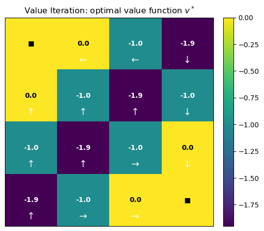
Optimal policy (arrows):
■ ← ← ↓
↑ ↑ ↑ ↓
↑ ↑ → ↓
↑ → → ■
5. Notes and Common Pitfalls
-
Step cost vs. terminal reward:
Using a constant step penalty (e.g., $r=-1$) encourages shortest-path behavior.
Whether the terminal transition gives $0$ or $-1$ mainly shifts all values by a constant — the optimal policy remains unchanged. -
Discount factor $\gamma$:
Larger $\gamma$ propagates future rewards farther across the state space, improving long-range planning but slowing convergence.
Smaller $\gamma$ yields faster convergence but more myopic behavior. -
Stopping tolerance $\theta$:
A loose tolerance may stop before true convergence; an extremely tight tolerance wastes computation.
In practice, choose $\theta$ based on the desired policy quality, not numerical perfection. -
Synchronous vs. in-place updates:
Synchronous value iteration is easier to reason about; in-place (Gauss–Seidel) updates often converge faster but are order-dependent.
RL Tie-In
This tabular algorithm is the exact solution later RL methods approximate:
- Q-learning / DQN ≈ sample-based value iteration on $Q(s,a)$ with function approximation
- Actor–Critic methods ≈ alternate between evaluation and improvement (policy iteration family)
- Neural targets in deep RL are direct analogs of the Bellman optimality backup used here
Understanding value iteration deeply makes modern RL algorithms feel like engineering extensions rather than new theory.
Key Takeaways
- Value Iteration repeatedly applies the Bellman optimality operator to converge to the optimal value function $v^*$.
- The maximum update $\Delta_k$ provides a simple, reliable convergence criterion; plotting it on a log scale reveals the contraction behavior clearly.
- The optimal policy is obtained by acting greedily with respect to $v^*$, selecting actions that maximize expected discounted return.
- This tabular dynamic programming procedure is the conceptual blueprint for later RL control methods that replace exact backups with sampled, approximate ones.
Next: 16_monte_carlo.ipynb → estimating values from episodic experience, without requiring a known transition model.