Basic Deep Learning
A practical intro to deep learning building blocks you’ll reuse in RL (policies, critics, world models).
What you’ll learn
- Neuron & activations (sigmoid, tanh, ReLU).
- MLP for classification (training loop, decision boundary).
- CNN for images (MNIST/Fashion-MNIST) with conv/pool layers.
- Regularization (Dropout, Weight Decay) & Normalization (BatchNorm).
- RL tie-ins: policies/critics, convolutional encoders for Atari, shared backbones.
Tip: Read each Theory cell first for context, then the code cells.
Setup
Code:
import math, time, numpy as np, matplotlib.pyplot as plt
import torch, torch.nn as nn, torch.nn.functional as F
from torch.utils.data import DataLoader, TensorDataset
from sklearn.datasets import make_moons
from sklearn.model_selection import train_test_split

device = torch.device("mps" if torch.backends.mps.is_available() else "cuda" if torch.cuda.is_available() else "cpu")
device
Output:
device(type='mps')
1. Neuron & Activations
At the heart of every neural network lies the neuron, a simple computational unit that performs a weighted sum followed by a nonlinear transformation:
\[y = \phi(w^\top x + b)\]where
- $ x \in \mathbb{R}^d $ is the input vector,
- $ w \in \mathbb{R}^d $ are learnable weights,
- $ b $ is a bias term, and
- $ \phi(\cdot) $ is the activation function introducing nonlinearity.
Common Activation Functions
-
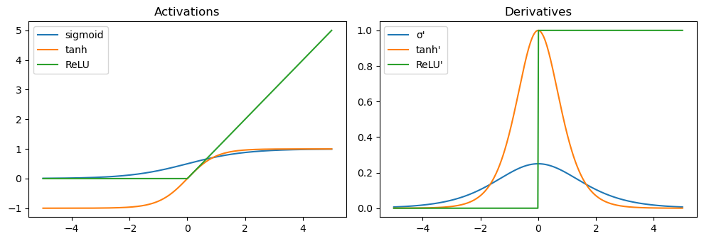
Sigmoid:
\[\sigma(z) = \frac{1}{1 + e^{-z}}\]Squashes values into (0, 1); good for probabilities but can saturate, leading to vanishing gradients.
-
tanh:
\[\tanh(z) = \frac{e^z - e^{-z}}{e^z + e^{-z}}\]Zero-centered but still saturates for large $|z|$.
-
ReLU (Rectified Linear Unit):
\[\text{ReLU}(z) = \max(0, z)\]Sparse activations, faster convergence, and widely used — though “dead neurons” can occur when gradients become zero.
From Neurons to Networks
Stacking layers of neurons forms a Multilayer Perceptron (MLP):
\[f(x) = W_L \,\phi(\cdots \phi(W_2\,\phi(W_1 x + b_1) + b_2)\cdots) + b_L\]Each layer learns progressively abstract features, enabling complex function approximation.
RL Connection
- In policy networks, the neuron layers map states $s$ to action probabilities $ \pi_\theta(a \mid s) $.
- In value networks, they estimate expected returns $V_\phi(s)$.
- Nonlinear activations (especially ReLU/tanh) allow the agent to capture nonlinear dynamics, enabling more expressive representations of policies and environment models.
Code:
# Visualizing activations and their derivatives
z = np.linspace(-5, 5, 500)
def sigmoid(z): return 1/(1+np.exp(-z))
def dsigmoid(z): s=sigmoid(z); return s*(1-s)
def tanh(z): return np.tanh(z)
def dtanh(z): t=np.tanh(z); return 1-t**2
def relu(z): return np.maximum(0,z)
def drelu(z): return (z>0).astype(float)

plt.figure(figsize=(10,3.5))
plt.subplot(1,2,1)
plt.plot(z, sigmoid(z), label="sigmoid"); plt.plot(z, tanh(z), label="tanh");
plt.plot(z, relu(z), label="ReLU")
plt.title("Activations"); plt.legend()

plt.subplot(1,2,2)
plt.plot(z, dsigmoid(z), label="σ'"); plt.plot(z, dtanh(z), label="tanh'");
plt.plot(z, drelu(z), label="ReLU'")
plt.title("Derivatives"); plt.legend()
plt.tight_layout(); plt.show()
2. MLP Classification on Moons
A Multilayer Perceptron (MLP) learns a nonlinear mapping from inputs $ x $ to class probabilities $ p_\theta(y \mid x) $. It consists of stacked fully connected layers with activations such as ReLU or tanh, followed by a softmax output layer for classification:
\[p_\theta(y=k \mid x) = \frac{e^{z_k}}{\sum_{j} e^{z_j}}, \quad \text{where } z = W_L h_{L-1} + b_L\]The network is trained by minimizing cross-entropy loss:
\[\mathcal{L}(\theta) = -\frac{1}{N}\sum_{i=1}^{N} \log p_\theta(y_i \mid x_i)\]This encourages the model to assign high probability to the correct class for each sample.
Practical Training Tips
- Use mini-batches to stabilize gradients and accelerate convergence.
- Monitor training vs validation loss to detect overfitting.
- Visualize decision boundaries to understand model behavior in low dimensions.
Reinforcement Learning Connection
In RL, policy networks often share the same architecture:
\[\pi_\theta(a \mid s) = \text{softmax}(W_2\,\phi(W_1 s + b_1) + b_2)\]where the MLP outputs probabilities over actions instead of class labels.
Here, minimizing cross-entropy mirrors maximizing policy likelihood in policy gradient methods. Similarly, the critic network can be viewed as a regression MLP estimating value functions.
Code:
# Data: two-moons
X, y = make_moons(n_samples=2000, noise=0.25, random_state=0)
X = X.astype(np.float32); y = y.astype(np.int64)
X_tr, X_te, y_tr, y_te = train_test_split(X, y, test_size=0.25, stratify=y, random_state=42)
train_dl = DataLoader(TensorDataset(torch.from_numpy(X_tr), torch.from_numpy(y_tr)), batch_size=64, shuffle=True)
test_dl = DataLoader(TensorDataset(torch.from_numpy(X_te), torch.from_numpy(y_te)), batch_size=256, shuffle=False)
class MLP(nn.Module):
def __init__(self, in_dim=2, hid=64, out_dim=2, pdrop=0.0, use_bn=False):
super().__init__()
layers = []
layers += [nn.Linear(in_dim, hid)]
if use_bn: layers += [nn.BatchNorm1d(hid)]
layers += [nn.ReLU(), nn.Dropout(pdrop)]
layers += [nn.Linear(hid, hid)]
if use_bn: layers += [nn.BatchNorm1d(hid)]
layers += [nn.ReLU(), nn.Dropout(pdrop)]
layers += [nn.Linear(hid, out_dim)]
self.net = nn.Sequential(*layers)
def forward(self, x): return self.net(x)
model = MLP(pdrop=0.1, use_bn=True).to(device)
opt = torch.optim.Adam(model.parameters(), lr=3e-3, weight_decay=1e-4) # weight decay = L2
loss_fn = nn.CrossEntropyLoss()
def run_epoch(dl, train=True):
model.train(train)
total, correct, n = 0.0, 0, 0
for xb, yb in dl:
xb, yb = xb.to(device), yb.to(device)
logits = model(xb)
loss = loss_fn(logits, yb)
if train:
opt.zero_grad(); loss.backward(); opt.step()
total += loss.item() * len(xb)
correct += (logits.argmax(dim=1)==yb).sum().item()
n += len(xb)
return total/n, correct/n
train_hist, test_hist = [], []
for epoch in range(40):
tr_loss, tr_acc = run_epoch(train_dl, train=True)
te_loss, te_acc = run_epoch(test_dl, train=False)
train_hist.append((tr_loss, tr_acc)); test_hist.append((te_loss, te_acc))
print({"train": train_hist[-1], "test": test_hist[-1]})
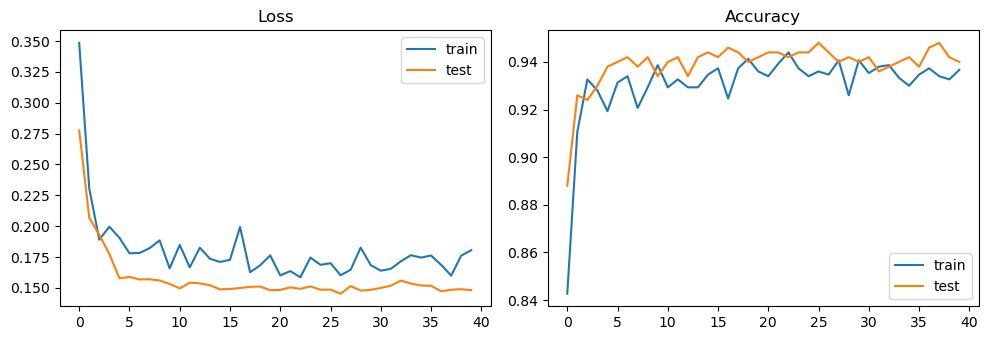
# Curves
plt.figure(figsize=(10,3.5))
plt.subplot(1,2,1); plt.plot([l for l,_ in train_hist], label="train");
plt.plot([l for l,_ in test_hist], label="test")
plt.title("Loss"); plt.legend()
plt.subplot(1,2,2); plt.plot([a for _,a in train_hist], label="train");
plt.plot([a for _,a in test_hist], label="test")
plt.title("Accuracy"); plt.legend(); plt.tight_layout(); plt.show()
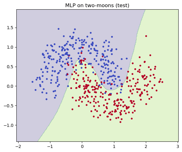
# Decision boundary
def plot_decision_boundary(model, X, y, title="Decision boundary"):
model.eval()
xv = np.linspace(X[:,0].min()-0.5, X[:,0].max()+0.5, 300)
yv = np.linspace(X[:,1].min()-0.5, X[:,1].max()+0.5, 300)
XX, YY = np.meshgrid(xv, yv)
grid = torch.from_numpy(np.c_[XX.ravel(), YY.ravel()].astype(np.float32)).to(device)
with torch.no_grad():
zz = model(grid).argmax(1).view(XX.shape).cpu().numpy()
plt.figure(figsize=(6,5))
plt.contourf(XX, YY, zz, levels=2, alpha=0.25)
plt.scatter(X[:,0], X[:,1], c=y, s=10, cmap="coolwarm")
plt.title(title); plt.tight_layout(); plt.show()
plot_decision_boundary(model, X_te, y_te, "MLP on two-moons (test)")
Output:
{'train': (0.18057496857643127, 0.9366666666666666), 'test': (0.14816934299468995, 0.94)}
3. CNN on MNIST
A Convolutional Neural Network (CNN) extends the MLP idea to spatial data (like images) by introducing convolutions — operations that exploit local spatial structure and reduce parameter count.
Core Building Blocks
-
Convolutional Layer: Each neuron looks at a small receptive field and applies shared filters:
\[y_{i,j,k} = \sum_{c} (W_{k,c} * X_c)_{i,j} + b_k\]where $ * $ denotes convolution, $W$ are learnable filters, and $b$ is bias.
-
Pooling: Reduces spatial size and increases translation invariance (e.g., MaxPool, AvgPool).
-
Nonlinearity: Applied after convolution — typically ReLU for fast and stable training.
-
Fully Connected Layers: After several conv+pool stages, flattened features feed into dense layers for classification.
Why CNNs Work
- Weight sharing: The same filter is used across the entire image — fewer parameters, better generalization.
- Spatial hierarchy: Lower layers learn edges/gradients; deeper ones capture shapes and objects.
- Translation tolerance: Pooling and local connectivity make the network robust to small shifts.
Reinforcement Learning Connection
- In Atari-style RL, agents observe raw pixels. CNNs act as feature extractors, mapping image frames $s_t$ → latent features $z_t$.
- These features then feed into:
- A policy head $ \pi_\theta(a \mid s) $ that outputs action probabilities.
- A value head $ V_\phi(s) $ estimating expected return.
- CNN encoders allow RL agents to learn from visual inputs directly, enabling breakthroughs in environments like Pong, Breakout, and DQN.
Code:
# Minimal CNN on MNIST
import torchvision
from torchvision import transforms
tfm = transforms.Compose([transforms.ToTensor()])
train_ds = torchvision.datasets.MNIST(root="./data", train=True, download=True, transform=tfm)
test_ds = torchvision.datasets.MNIST(root="./data", train=False, download=True, transform=tfm)
train_loader = DataLoader(train_ds, batch_size=128, shuffle=True, num_workers=0)
test_loader = DataLoader(test_ds, batch_size=256, shuffle=False, num_workers=0)
class SmallCNN(nn.Module):
def __init__(self, num_classes=10):
super().__init__()
self.feat = nn.Sequential(
nn.Conv2d(1, 32, 3, padding=1), nn.ReLU(),
nn.MaxPool2d(2), # 14x14
nn.Conv2d(32, 64, 3, padding=1), nn.ReLU(),
nn.MaxPool2d(2), # 7x7
)
self.head = nn.Sequential(
nn.Flatten(),
nn.Linear(64*7*7, 128), nn.ReLU(),
nn.Dropout(0.2),
nn.Linear(128, num_classes)
)
def forward(self, x):
return self.head(self.feat(x))
cnn = SmallCNN().to(device)
opt_cnn = torch.optim.Adam(cnn.parameters(), lr=1e-3)
ce = nn.CrossEntropyLoss()
def epoch_loop(model, loader, train=True):
model.train(train)
total, correct, n = 0.0, 0, 0
for xb, yb in loader:
xb, yb = xb.to(device), yb.to(device)
logits = model(xb)
loss = ce(logits, yb)
if train:
opt_cnn.zero_grad(); loss.backward(); opt_cnn.step()
total += loss.item() * len(xb)
correct += (logits.argmax(1)==yb).sum().item()
n += len(xb)
return total/n, correct/n
mnist_hist = {"train": [], "test": []}
for ep in range(5): # keep it light; bump to 10–15 for stronger accuracy
tr = epoch_loop(cnn, train_loader, True)
te = epoch_loop(cnn, test_loader, False)
mnist_hist["train"].append(tr); mnist_hist["test"].append(te)
print("MNIST final:", {"train": mnist_hist["train"][-1], "test": mnist_hist["test"][-1]})
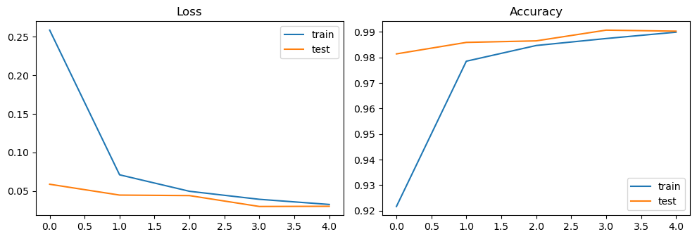
plt.figure(figsize=(10,3.5))
plt.subplot(1,2,1); plt.plot([l for l,_ in mnist_hist["train"]], label="train");
plt.plot([l for l,_ in mnist_hist["test"]], label="test"); plt.title("Loss"); plt.legend()
plt.subplot(1,2,2); plt.plot([a for _,a in mnist_hist["train"]], label="train");
plt.plot([a for _,a in mnist_hist["test"]], label="test"); plt.title("Accuracy"); plt.legend()
plt.tight_layout(); plt.show()
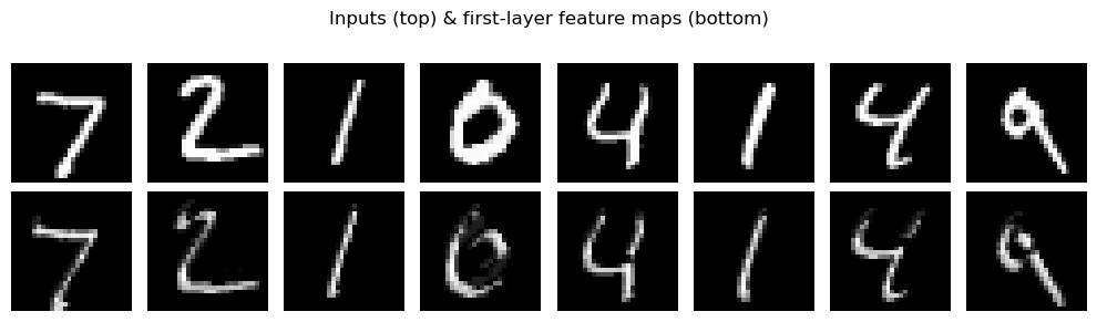
# Peek feature maps
xb, yb = next(iter(test_loader))
xb = xb[:8].to(device)
with torch.no_grad():
fm = cnn.feat[:2](xb) # after first Conv+ReLU
fm = fm.cpu().numpy()
plt.figure(figsize=(10,3))
for i in range(8):
plt.subplot(2,8,i+1); plt.imshow(xb[i,0].cpu(), cmap="gray"); plt.axis("off")
plt.subplot(2,8,8+i+1); plt.imshow(fm[i,0], cmap="gray"); plt.axis("off")
plt.suptitle("Inputs (top) & first-layer feature maps (bottom)")
plt.tight_layout(); plt.show()
Output:
MNIST final: {'train': (0.03260704416930676, 0.9899), 'test': (0.030221648491127417, 0.9903)}
4. Regularization & Normalization
Deep networks can easily overfit or suffer from unstable optimization. Regularization and normalization techniques mitigate these problems and improve generalization.
Weight Decay (L2 Regularization)
Adds a penalty proportional to the squared magnitude of the weights:
\[\mathcal{L}_{\text{total}} = \mathcal{L}_{\text{task}} + \lambda \|W\|_2^2\]This discourages large weights, improving numerical stability and reducing overfitting. Modern optimizers (e.g., AdamW) decouple weight decay from gradient updates for better control.
Dropout
Randomly “drops” activations during training with probability $p$:
\[h_i' = \begin{cases} 0, & \text{with prob } p,\\[6pt] \frac{h_i}{1-p}, & \text{otherwise.} \end{cases}\]This prevents neurons from co-adapting too strongly and acts as an implicit ensemble.
Batch Normalization
Normalizes intermediate activations within each batch:
\[\hat{x} = \frac{x - \mu_{\text{batch}}}{\sigma_{\text{batch}}}, \quad y = \gamma \hat{x} + \beta\]This reduces internal covariate shift, leading to smoother gradients and faster convergence.
RL Connection
- Weight Decay: used in nearly all deep RL architectures (DQN, PPO, SAC) for stability.
- Dropout: helps in policy regularization and exploration in small fully connected nets.
- BatchNorm / LayerNorm: stabilize feature distributions in value critics and transformer-based policies. (For instance, PPO and Dreamer often use LayerNorm in latent models.)
In short: Regularization prevents overfitting, normalization stabilizes learning — both are pillars of reliable deep and reinforcement learning.
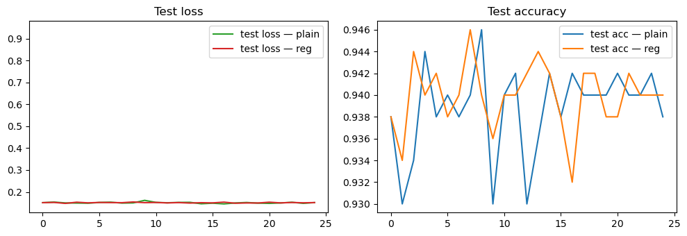
Code:
# Quick comparison: MLP with/without Dropout & Weight Decay (two-moons)
def train_mlp(pdrop=0.0, wd=0.0):
    m = MLP(pdrop=pdrop, use_bn=False).to(device)
    optm = torch.optim.AdamW(m.parameters(), lr=3e-3, weight_decay=wd)
    hist=[]
    for ep in range(25):
        tr = run_epoch(DataLoader(TensorDataset(torch.from_numpy(X_tr), torch.from_numpy(y_tr)), batch_size=64,
        shuffle=True), True)
        te = run_epoch(DataLoader(TensorDataset(torch.from_numpy(X_te), torch.from_numpy(y_te)), batch_size=256,
        shuffle=False), False)
        hist.append((tr, te))
    return m, hist

m_plain, h_plain = train_mlp(pdrop=0.0, wd=0.0)
m_reg,   h_reg   = train_mlp(pdrop=0.2, wd=1e-3)

plt.figure(figsize=(10,3.5))
plt.subplot(1,2,1)
plt.plot([te for (_,te) in [h_plain[-1], h_reg[-1]]], alpha=0) # spacer
plt.plot([l for l,_ in [x[1] for x in h_plain]], label="test loss — plain")
plt.plot([l for l,_ in [x[1] for x in h_reg]],   label="test loss — reg")
plt.title("Test loss"); plt.legend()

plt.subplot(1,2,2)
plt.plot([a for _,a in [x[1] for x in h_plain]], label="test acc — plain")
plt.plot([a for _,a in [x[1] for x in h_reg]],   label="test acc — reg")
plt.title("Test accuracy"); plt.legend()
plt.tight_layout(); plt.show()
Key Takeaways
- Neurons & Activations: ReLU/tanh give nonlinearity; choose activations to keep gradients healthy.
- MLPs & CNNs: MLPs for low-dim states; CNNs for pixels. Training = forward → loss → backward → step.
- Regularization: Weight decay, Dropout, and normalization improve generalization & stability.
- Direct RL relevance: These modules become policy/critic heads and encoders in RL.
Next: 08_introduction_to_markov_chains.ipynb → states, transitions, stationary distributions (foundation for MDPs).