PyTorch Basics
From tensors and autograd to training your first MLP — the essentials for deep RL.
What you’ll learn
torch.Tensorand autograd (automatic differentiation)- Building models with
nn.Module/nn.Sequential - Losses, optimizers (SGD, Adam), and training loops
- Classification & regression mini‑examples
- Plotting learning curves
Policies and value functions in deep RL are just neural networks trained with these fundamentals (e.g., PPO actor & critic).
Code:
import numpy as np
import matplotlib.pyplot as plt

import torch
import torch.nn as nn
import torch.nn.functional as F
from torch.utils.data import TensorDataset, DataLoader

torch.manual_seed(0)
if torch.cuda.is_available():
    device = torch.device("cuda")
elif torch.backends.mps.is_available():
    device = torch.device("mps")
else:
    device = torch.device("cpu")

print(f"Using device: {device}")
Output:
Using device: mps
1. Autograd in a Nutshell
PyTorch’s autograd system automatically computes derivatives of tensor operations using reverse-mode differentiation, the same principle behind backpropagation.
When a tensor is created with
x = torch.tensor([...], requires_grad=True)
PyTorch records all operations on it in a computation graph. When you call .backward(), it traverses this graph in reverse to compute gradients efficiently.
Mathematical Intuition
For a scalar function
\[y = f(x_1, x_2, \dots, x_n),\]autograd computes
\[\frac{\partial y}{\partial x_i}\]for each parameter via the chain rule:
\[\frac{\partial y}{\partial x_i} = \sum_j \frac{\partial y}{\partial z_j} \frac{\partial z_j}{\partial x_i}.\]In vector form, this becomes efficient reverse-mode differentiation, ideal when the number of outputs ≪ number of parameters — exactly the case in neural networks.
RL Connection
- Policy networks, value functions, and Q-networks all rely on autograd for computing
- \[\nabla_\theta J(\pi_\theta) = \mathbb{E}*\pi [\nabla*\theta \log \pi_\theta(a \mid s) , G_t].\]
- Autograd automates gradient computation for loss functions like:
- Policy gradient loss
- Temporal-difference (TD) error
- Actor-critic combined objectives
- This makes it easy to experiment and debug custom RL algorithms without manual gradient derivations.
Code:
# Define tensors with gradient tracking enabled
x = torch.tensor([2.0, -1.0], requires_grad=True)
w = torch.tensor([1.5, -3.0], requires_grad=True)
b = torch.tensor(0.5, requires_grad=True)

# Forward pass: simple linear model y = w·x + b
y = torch.dot(w, x) + b

# Backward pass: compute gradients dy/dx, dy/dw, dy/db
y.backward()

print(f"Output y: {y.item():.3f}")
print("dy/dx:", x.grad)
print("dy/dw:", w.grad)
print("dy/db:", b.grad)
Output:
Output y: 6.500
dy/dx: tensor([ 1.5000, -3.0000])
dy/dw: tensor([ 2., -1.])
dy/db: tensor(1.)
2. A Tiny MLP for Classification
A Multi-Layer Perceptron (MLP) is a feedforward neural network composed of linear layers and nonlinear activations. It learns a function $ f_\theta: \mathbb{R}^n \to \mathbb{R}^k $ by minimizing a loss (e.g., cross-entropy for classification).
Structure
For an input $x \in \mathbb{R}^n$:
\[h_1 = \sigma(W_1 x + b_1), \quad \hat{y} = \text{softmax}(W_2 h_1 + b_2)\]where:
- $W_i, b_i$ are learnable parameters,
- $\sigma(\cdot)$ is a nonlinear activation (e.g., ReLU, tanh),
- The softmax maps logits to class probabilities.
The model learns by minimizing:
\[\mathcal{L}(\theta) = -\frac{1}{N}\sum_{i=1}^N y_i^\top \log \hat{y}_i\]using stochastic gradient descent or Adam.
Intuition
Each layer transforms the input into a more linearly separable space.
Nonlinear activations allow the network to represent complex decision boundaries.
RL Connection
- Policy networks and Q-networks in RL are often MLPs mapping states to:
- Action probabilities (policy output via softmax)
- Value estimates $ V_\theta(s) $
- The same forward-backward mechanics apply:
- Forward pass → compute predicted reward/value.
- Backward pass → compute gradient and update parameters.
Code:
# Reproducibility
np.random.seed(0)
torch.manual_seed(0)
# Data: two Gaussian blobs
n_per = 300
cov = 0.3 * np.eye(2)
X0 = np.random.multivariate_normal([0, 0], cov, size=n_per)
X1 = np.random.multivariate_normal([2, 2], cov, size=n_per)
X = np.vstack([X0, X1]).astype(np.float32)
y = np.concatenate([np.zeros(n_per), np.ones(n_per)]).astype(np.int64)
# Convert to tensors and build loader
X_t = torch.from_numpy(X)
y_t = torch.from_numpy(y)
ds = TensorDataset(X_t, y_t)
dl = DataLoader(ds, batch_size=64, shuffle=True)
# Model
class MLP(nn.Module):
def __init__(self):
super().__init__()
self.net = nn.Sequential(
nn.Linear(2, 32),
nn.ReLU(),
nn.Linear(32, 2)
)
def forward(self, x):
return self.net(x)
print("Using device: ", device)
model = MLP().to(device)
opt = torch.optim.Adam(model.parameters(), lr=1e-2)
criterion = nn.CrossEntropyLoss()
# Train
loss_hist = []
for epoch in range(30):
model.train()
running = 0.0
for xb, yb in dl:
xb, yb = xb.to(device), yb.to(device)
opt.zero_grad()
logits = model(xb)
loss = criterion(logits, yb)
loss.backward()
opt.step()
running += loss.item() * len(xb)
loss_hist.append(running / len(ds))
# Evaluate accuracy
model.eval()
with torch.no_grad():
logits = model(X_t.to(device))
y_pred = torch.argmax(logits, dim=1).cpu().numpy()
acc = (y_pred == y).mean()
print(f"Training accuracy: {acc:.4f}")
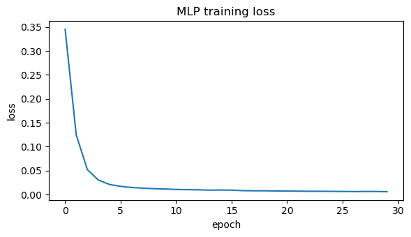
# Plot loss
plt.figure(figsize=(6,3.5))
plt.plot(loss_hist)
plt.title("MLP training loss")
plt.xlabel("epoch"); plt.ylabel("loss")
plt.tight_layout(); plt.show()
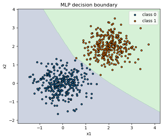
# Decision boundary visualization
pad = 0.5
x_min, x_max = X[:,0].min() - pad, X[:,0].max() + pad
y_min, y_max = X[:,1].min() - pad, X[:,1].max() + pad
xx, yy = np.meshgrid(np.linspace(x_min, x_max, 300),
np.linspace(y_min, y_max, 300))
grid = np.c_[xx.ravel(), yy.ravel()].astype(np.float32)
with torch.no_grad():
logits_grid = model(torch.from_numpy(grid).to(device))
pred_grid = torch.argmax(logits_grid, dim=1).cpu().numpy().reshape(xx.shape)
plt.figure(figsize=(5.6,4.8))
plt.contourf(xx, yy, pred_grid, alpha=0.25, levels=[-0.5,0.5,1.5])
plt.scatter(X0[:,0], X0[:,1], s=16, label="class 0", edgecolor="k")
plt.scatter(X1[:,0], X1[:,1], s=16, label="class 1", edgecolor="k")
plt.title("MLP decision boundary")
plt.xlabel("x1"); plt.ylabel("x2"); plt.legend()
plt.tight_layout(); plt.show()
Output:
Using device:  mps
Training accuracy: 1.0000
3. Regression with MSE
In regression, the goal is to predict a continuous target $ y \in \mathbb{R} $ from input features $ x \in \mathbb{R}^n $. A neural model (or any differentiable function) $ f_\theta(x) $ is trained by minimizing the Mean Squared Error (MSE):
\[\mathcal{L}(\theta) = \frac{1}{N} \sum_{i=1}^{N} \big(f_\theta(x_i) - y_i\big)^2\]Here:
- $ f_\theta(x) $ → predicted value
- $ y_i $ → ground truth
- The gradient w.r.t. parameters $ \theta $ points toward reducing the prediction error.
Intuition
The model learns to fit a regression line (or surface) through the data that minimizes squared deviations between predictions and actual values.
Unlike classification, the output layer here is linear (no softmax or sigmoid).
RL Connection
- In value function approximation, the critic predicts expected returns $ V_\theta(s) $.
-
The training signal comes from bootstrapped targets, e.g.:
\[\mathcal{L}(\theta) = \mathbb{E}\big[(r_t + \gamma V_\theta(s_{t+1}) - V_\theta(s_t))^2\big]\] - This is the same MSE objective, but the targets are dynamic (changing as learning progresses).
Understanding regression with MSE provides the mathematical and coding foundation for critic updates, Q-learning, and actor-critic algorithms in deep reinforcement learning.
Code:
# Synthetic data: y = 2x - 3 + noise
xs = np.linspace(-2, 2, 200, dtype=np.float32).reshape(-1, 1)
ys = (2 * xs - 3 + 0.3 * np.random.randn(*xs.shape)).astype(np.float32)
Xt = torch.from_numpy(xs).to(device)
Yt = torch.from_numpy(ys).to(device)
# Model: small MLP (can fit linear smoothly)
reg = nn.Sequential(
nn.Linear(1, 32),
nn.ReLU(),
nn.Linear(32, 1)
).to(device)
print("Using device: ", device)
opt = torch.optim.SGD(reg.parameters(), lr=1e-2, momentum=0.9)
mse = nn.MSELoss()
# Train
losses = []
for epoch in range(200):
opt.zero_grad()
pred = reg(Xt)
loss = mse(pred, Yt)
loss.backward()
opt.step()
losses.append(loss.item())
# Metrics: MSE & R^2 on full dataset
with torch.no_grad():
yp = reg(Xt).cpu().numpy()
mse_val = float(np.mean((ys - yp)**2))
ss_res = float(np.sum((ys - yp)**2))
ss_tot = float(np.sum((ys - ys.mean())**2))
r2 = 1.0 - ss_res / ss_tot
print(f"MSE: {mse_val:.4f} R^2: {r2:.4f}")
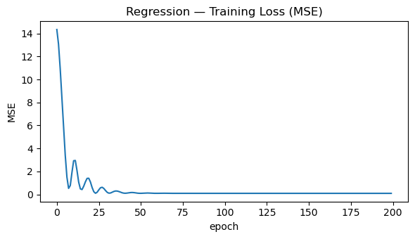
# Plot training loss
plt.figure(figsize=(6, 3.5))
plt.plot(losses)
plt.title("Regression — Training Loss (MSE)")
plt.xlabel("epoch"); plt.ylabel("MSE")
plt.tight_layout(); plt.show()
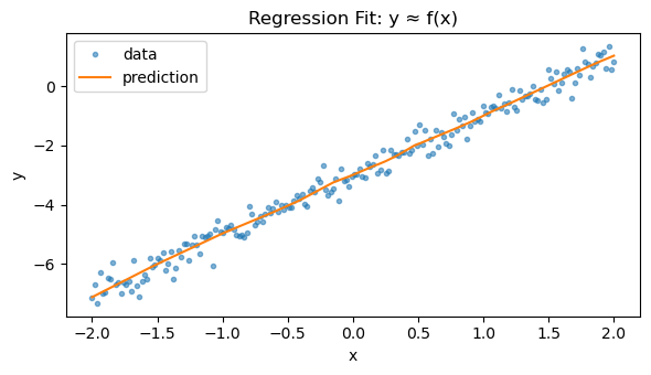
# Visualize fit
plt.figure(figsize=(6, 3.5))
plt.plot(xs, ys, ".", alpha=0.55, label="data")
plt.plot(xs, yp, "-", label="prediction")
plt.title("Regression Fit: y ≈ f(x)")
plt.xlabel("x"); plt.ylabel("y")
plt.legend(); plt.tight_layout(); plt.show()
Output:
Using device:  mps
MSE: 0.0905   R^2: 0.9838
Key Takeaways
- Autograd — PyTorch automatically computes gradients via backpropagation.
- nn.Module & Optimizers — Simplify model definition and parameter updates.
- Foundation for RL — Core of policy, value, and world model training in deep RL.
Next: 05_gymnasium_basics.ipynb → explore RL environments and agent–environment loops.